Graphical Methods and Interpretation – plotting, analysis, and business applications

Graphical Methods and Interpretation

1. Coordinate System and Plotting

A Cartesian plane consists of an x‑axis (horizontal) and a y‑axis (vertical).

• The intersection point is the origin $(0,0)$.
• Units are equally spaced along each axis.

Plotting a point $(a,b)$: locate $a$ units along the x‑axis, then $b$ units vertically.

2. Linear Functions

A linear function has the form
$$y=mx+b,$$
where $m$ is the slope and $b$ the y‑intercept.

• Slope $m=\frac{\Delta y}{\Delta x}$ represents the rate of change.
• Intercepts: $x$-intercept when $y=0$; $y$-intercept when $x=0$.

Example: For $y=2x+3$, the slope $m=2$ indicates that for every unit increase in $x$, $y$ increases by 2 units.

3. Quadratic Functions

A quadratic function is
$$y=a{x}^2+bx+c,$$
with $a\ne 0$.

• Vertex $\left(-\frac{b}{2a},c-\frac{b^2}{4a}\right)$.
• Axis of symmetry $x=-\frac{b}{2a}$.
• Direction: opens upward if $a>0$, downward if $a<0$.

Interpretation: The vertex gives the maximum or minimum value, useful for profit maximization or cost minimization.

4. Exponential and Logarithmic Functions

• Exponential: $y=a{b}^x$ with $b>0,b\ne 1$.
  • Growth if $b>1$; decay if $0<b<1$.
• Logarithmic: $y={\log }_{b}x$ is the inverse of the exponential.

Business relevance: Compound interest, population growth, depreciation.

5. Piecewise Functions

Defined by different expressions over intervals.

Interpretation: Models step‑wise pricing, tax brackets, or service tiers.

6. Parametric and Polar Graphs

• Parametric: $x=f(t),y=g(t)$.
• Polar: $r=f(\theta )$.

Applications: Circular motion, oscillations, radar plots.

7. Transformations of Graphs

• Translation: $(x-h,y-k)$.
• Scaling: Multiply $x$ or $y$ by a factor.
• Reflection: Across axes or lines.

Business use: Adjusting cost curves for inflation (vertical shift) or scaling production volumes (horizontal stretch).

8. Interpretation of Graphs

9. Graphical Solution of Systems

Plot each equation; the intersection point(s) satisfy all equations.

Worked Example:
Solve
$$\{\begin{array}{l}y=2x+3,\\ y=-x+5.\end{array}$$
Intersection at $(1,5)$.

10. Linear Programming – Feasible Region

Constraints are linear inequalities.

• Feasible region: set of all points satisfying all constraints.
• Objective function: linear expression to maximize or minimize.

Corner Point Method: Evaluate the objective function at each vertex of the feasible region.

flowchart TD
  A["Plot constraints"] --> B["Identify feasible region"]
  B --> C["Find vertices (corner points)"]
  C --> D["Compute objective at each vertex"]
  D --> E["Select maximum (or minimum) value"]

Worked Example:
Maximize $Z=5x_1+3x_2$
subject to
$$\{\begin{array}{l}2x_1+x_2\le 5,\\ x_1+x_2\le 4,\\ x_1,x_2\ge 0.\end{array}$$

Feasible vertices: $(0,0),(0,4),(2,1),(1,3)$.
$Z$ values: $0,12,13,12$.
Optimal solution: $(2,1)$ with $Z=13$.

11. Business Applications

Worked Example – Demand & Supply Equilibrium

Demand: $Q_d=26-0.4P$
Supply: $Q_s=4+0.6P$

Set $Q_d=Q_s$:
$$26-0.4P=4+0.6P⟹22=P⟹P^{\ast }=22.$$
Equilibrium quantity: $Q^{\ast }=26-0.4(22)=14.8$.

Graphically, the intersection of the two lines confirms the equilibrium.

Worked Example – Daraz Order Queue (Linear Programming)

Objective: Maximize daily order processing $Z=10x_1+8x_2$
where $x_1$ = number of express vans, $x_2$ = number of standard vans.
Constraints:

• Total vans ≤ 20.
• Express vans ≤ 12.
• Standard vans ≤ 15.
• Each express van processes 10 orders/day, standard 8 orders/day.

Feasible region vertices: $(0,0),(12,0),(0,15),(12,8)$.
Compute $Z$:

• $(12,8)$: $Z=10(12)+8(8)=120+64=184$.
  Optimal: 12 express + 8 standard vans → 184 orders/day.

Worked Example – Kathmandu Traffic Route (Shortest Path)

Model traffic network as a graph with nodes (intersections) and weighted edges (travel time).
Use Dijkstra’s algorithm (graph theory).
Result: shortest route from Patan to Pokhara takes 2 hours via Kirtipur and Bhairahawa.

12. Comparison Table: Graphical vs Algebraic Methods

13. Advantages and Disadvantages

14. In the real world

• eSewa transaction volume vs time: A line graph of daily transaction counts shows peak hours; the slope indicates surge rate.
• Daraz order queue: The linear programming model above directly informs how many vans to deploy each shift.
• Kathmandu traffic routes: The shortest‑path graph determines optimal detours during peak traffic, improving delivery times.
• NEPSE price adjustment: The demand‑supply equilibrium graph helps traders anticipate price movements during market openings.

15. Exam tip

• Identify the type of graph (linear, quadratic, exponential, piecewise) before sketching.
• Mark intercepts and slopes; they are often the key to solving problems.
• For LP problems, draw the feasible region, label corner points, and evaluate the objective at each.
• Check units: In business contexts, units (Rs, orders, time) matter for interpretation.
• Practice converting equations to graph form; this speeds up sketching and analysis.

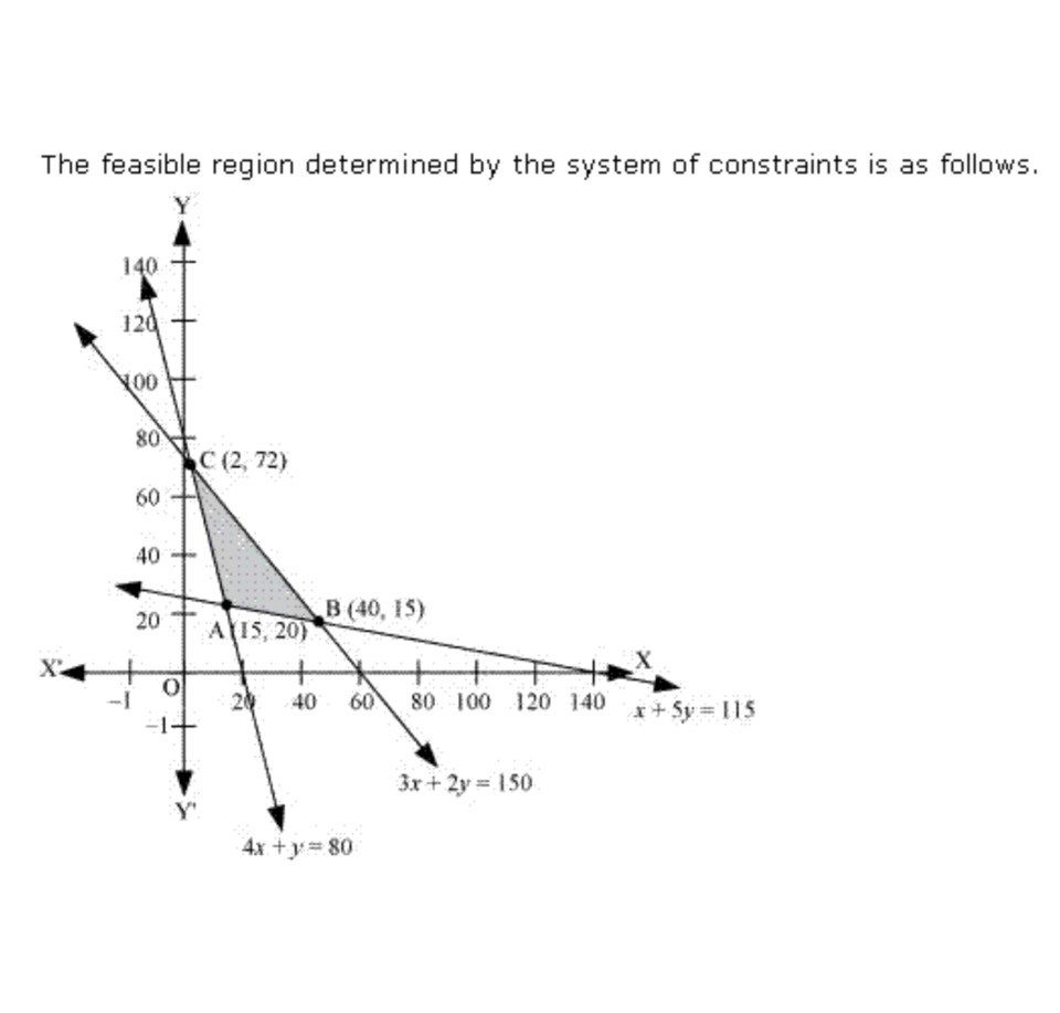Feasible region for LP problem (Image: Lpp3535, CC BY-SA 4.0, via Wikimedia Commons)