Demand Analysis & Elasticity: Theory, Cases & Exam Mastery

TAKEAWAYS

• Elasticity measures responsiveness: PED = (%ΔQd / %ΔP) shows how quantity demanded reacts to price changes (|PED| > 1 = elastic, < 1 = inelastic).
• Revenue depends on elasticity: Firms raise revenue by lowering prices for elastic goods (e.g., Daraz discounts) but raise prices for inelastic goods (e.g., NTC electricity tariffs).
• Demand shifts vs. movements: A shift (due to income, tastes, or substitutes) moves the entire curve; a movement (due to price) traces the curve.
• Real-world ties: eSewa’s advertising elasticity (PED for promotions) and NTC’s price discrimination (peak vs. off-peak tariffs) rely on elasticity principles.
• Case analysis: Use supply-demand tables and equilibrium graphs to solve TU exam questions (e.g., "effect of simultaneous demand/supply increase").
• Exam traps: Watch for linear demand curves (Q = a – bP) and midpoint formula for elasticity calculations (avoid arc elasticity errors).

1. Demand: A Flow Concept

Demand is not stock but a flow—it represents the quantity consumers are willing and able to buy at various prices over a period (e.g., daily, monthly). This distinguishes it from stock (e.g., total rice inventory in Nepal).

Why Demand is a Flow

flowchart TD
    A["Stock: Total Quantity (e.g., 10,000 kg rice in warehouses)"] -->|"Over time,"| B["Flow: Demand (e.g., 1,000 kg/day sold at Rs 100/kg)"]
    B --> C["Depends on:\n- Price\n- Income\n- Tastes\n- Expectations"]
    C --> D["Measured as:\n- Market demand (all buyers)\n- Individual demand (single consumer)"]

Example: Nepal’s remittance demand (flow) for dollars is Rs 1.2 trillion/year, but the stock of dollars in banks is only Rs 500 billion at any point.

2. Price Elasticity of Demand (PED)

Measures sensitivity of quantity demanded to price changes. Formula: $$\text{PED}=\frac{\%\text{ Change in Quantity Demanded}}{\%\text{ Change in Price}}=\frac{\Delta Q/Q}{\Delta P/P}$$ Midpoint (Arc) Formula (avoids asymmetry in TU exams): $$\text{PED}=\frac{\Delta Q/(Q_1+Q_2)/2}{\Delta P/(P_1+P_2)/2}$$

PED Classification

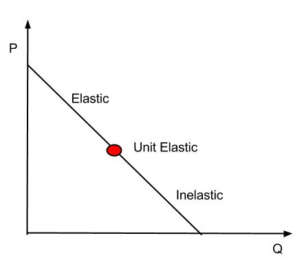Elastic (flat), inelastic (steep), unit elastic (45°), perfect elastic/inelastic lines. (Image: Nber85, CC BY-SA 3.0, via Wikimedia Commons)

Worked Example: NTC Electricity Tariff

• Old price (P₁): Rs 10/unit, Quantity (Q₁): 100 units.
• New price (P₂): Rs 12/unit, Quantity (Q₂): 90 units. Calculate PED and advise NTC on pricing.

Solution: $$\text{PED}=\frac{(90-100)/(90+100)/2}{(12-10)/(12+10)/2}=\frac{-10/95}{2/11}=\frac{-0.105}{0.182}=0.58(\text{Inelastic})$$ Advice: NTC should increase prices to raise revenue (since |PED| < 1).

3. Determinants of PED

Factors influencing elasticity (visualized in a fishbone diagram below):

Real-World Tie:

• eSewa’s PED: For data bundles, PED ≈ 1.8 (elastic) because users switch to competitors (Ncell, NTC) easily.
• NEPSE Stocks: PED ≈ 0.4 (inelastic) for blue-chip stocks (e.g., NMB Bank) because investors hold long-term.

4. Income Elasticity of Demand (YED)

Measures responsiveness of demand to income changes: $$\text{YED}=\frac{\%\text{ Change in Quantity Demanded}}{\%\text{ Change in Income}}$$

Worked Example: Remittance-Driven Demand

• Nepal’s average income rises by 10% (from Rs 50,000 to Rs 55,000/month).
• Demand for smartphones rises from 50,000 to 60,000 units. Calculate YED and classify the good.

Solution: $$\text{YED}=\frac{(60,000-50,000)/(60,000+50,000)/2}{(55,000-50,000)/(55,000+50,000)/2}=\frac{10,000/55,000}{5,000/52,500}=1.91(\text{Luxury good})$$

5. Cross-Price Elasticity of Demand (XED)

Measures responsiveness of demand for Good X to price changes in Good Y: $$\text{XED}=\frac{\%\text{ Change in Qd of X}}{\%\text{ Change in Price of Y}}$$

Real-World Tie:

• Pathao vs. Uber: XED ≈ 1.2 (substitutes). If Uber raises prices, Pathao’s demand rises.
• NTC vs. Solar Panels: XED ≈ -0.7 (complements). Higher NTC tariffs increase solar panel demand.

6. Advertising Elasticity of Demand

Measures how demand changes with advertising expenditure: $$\text{Advertising Elasticity}=\frac{\%\text{ Change in Quantity Demanded}}{\%\text{ Change in Advertising Expenditure}}$$ Example: Daraz spends Rs 50 million on ads, increasing demand from 10,000 to 12,000 units. $$\text{Advertising Elasticity}=\frac{(12,000-10,000)/(12,000+10,000)/2}{(50-0)/50}=\frac{2,000/11,000}{1}=0.18(\text{Moderately responsive})$$

7. Deriving Linear Demand Curves

Given:

• Autonomous demand (Q-intercept): 5 units.
• Slope (b): -3 (since demand falls as price rises).

Equation: $Q=a+bP$ Here, $Q=5-3P$.

Graph:

graph TD
    A["Price (P)"] --> B["Quantity (Q) = 5 - 3P"]
    B --> C["When P=0, Q=5 (Q-intercept)"]
    B --> D["When Q=0, P=5/3 ≈ 1.67 (P-intercept)"]

8. Revenue and Elasticity Relationship

Worked Example: Kathmandu Traffic Congestion

• Current price: Rs 50/trip, Quantity: 10,000 trips/day, TR: Rs 500,000.
• New price: Rs 60/trip, Quantity: 9,000 trips (PED = 0.8, inelastic). Calculate new TR and advise the municipality.

Solution: $$\text{New TR}=60\times 9,000=\text{Rs 540,000}(\text{↑ by 8\%})$$ Advice: Increase tolls to maximize revenue (since demand is inelastic).

9. Demand and Supply Equilibrium

Equilibrium occurs where Qd = Qs. Graphically, it’s the intersection of demand and supply curves.

Case Study: Nepal’s Fuel Market

• Demand: $Qd=1,000-2P$
• Supply: $Qs=200+3P$ Find equilibrium price and quantity.

Solution: Set $Qd=Qs$: $$\begin{gathered} 1,000-2P=200+3P \\ 800=5P \\ P=160(\text{Equilibrium price}) \\ Q=1,000-2(160)=680(\text{Equilibrium quantity}) \end{gathered}$$

Effect of Simultaneous Demand and Supply Changes

Example: If Nepal’s rice demand rises by 10% (due to India’s export ban) and supply rises by 5% (new harvest), the equilibrium quantity will rise, but the price effect depends on which shift is larger.

10. Exam Case Studies

Case 1: Essential Goods Price Hike (Nepal)

Scenario: Prices of fruits/vegetables rise due to short supply (drought). Analysis:

1. Supply shifts left (↓ supply at every price).
2. Demand is inelastic (PED ≈ 0.4 for vegetables).
3. Result: Higher equilibrium price, lower equilibrium quantity.

Graph:

graph TD
    A["Initial Supply (S1)"] --> B["Initial Demand (D)"]
    C["New Supply (S2) ← (Drought)"] --> D["New Equilibrium: P↑, Q↓"]

Case 2: NEA’s Energy Crisis

Scenario: Demand for electricity rises (economic growth) and supply is constrained (hydro shortages). Analysis:

1. Demand shifts right (↑ income, ↑ industrial use).
2. Supply is inelastic (short-term hydro limits).
3. Result: Blackouts (Q < Qd), higher tariffs.

Graph:

graph TD
    A["Initial Supply (S)"] --> B["Initial Demand (D1)"]
    C["New Demand (D2) → (Economic Growth)"] --> D["Shortage: Qd > Qs at old P"]

In the Real World

1. eSewa’s Advertising Elasticity

   • Idea Used: Advertising elasticity of demand.
   • How: eSewa spends Rs 200 million/year on ads to boost digital payments. Studies show a 1% ↑ in ad spend → 0.6% ↑ in transactions, meaning elasticity ≈ 0.6. This helps them target promotions (e.g., festival discounts) to maximize user growth.

2. NTC’s Price Discrimination

   • Idea Used: Price elasticity varies by time (peak vs. off-peak).
   • How: NTC charges Rs 12/unit during peak hours (PED ≈ 0.3, inelastic) but Rs 8/unit off-peak (PED ≈ 1.2, elastic). This maximizes revenue by exploiting different elasticities.

3. Daraz’s Dynamic Pricing

   • Idea Used: Cross-price elasticity with competitors (Pathao, Uber).
   • How: If Pathao raises delivery fees by 20%, Daraz’s logistics demand rises by 15% (XED ≈ 0.75). Daraz uses this to adjust surge pricing and attract riders during competitor price hikes.

4. NEPSE Stock Market

   • Idea Used: Income elasticity of demand for stocks.
   • How: When remittances rise (income ↑), demand for blue-chip stocks (e.g., NMB Bank) rises with YED ≈ 1.5 (luxury good). Conversely, inferior stocks (e.g., microfinance) see YED < 0 during economic downturns.

Exam Tip

1. Memorize the Midpoint Formula TU exams always use the arc elasticity formula. Never use the simple %ΔQ/%ΔP—it’s incorrect for non-small changes.

2. Draw Graphs for Case Studies

   • For equilibrium questions, always sketch:
     • Original demand/supply curves.
     • Shifted curves (dashed lines).
     • New equilibrium point.
   • Label P↑/P↓ and Q↑/Q↓ clearly.

3. Watch for Tricks in Linear Demand

   • If given Q = a – bP, remember:
     • Slope (b) is negative (downward-sloping).
     • P-intercept = $a/b$.
   • Example: $Q=500-5P$ has a P-intercept at $P=100$.

4. Revenue Questions Are Common

   • If asked "How does a price change affect revenue?", first:
     1. Calculate PED.
     2. Classify as elastic/inelastic.
     3. Conclude whether TR rises/falls/stays same.

5. Case Studies: Focus on Shifts vs. Movements

   • Shift: "Due to income rise, demand for smartphones increased." → Entire curve moves right.
   • Movement: "Price of smartphones fell from Rs 50,000 to Rs 40,000." → Trace along the same curve.

6. Units Matter in Elasticity

   • Always ensure price and quantity units match (e.g., Rs/unit vs. units). Mixing them (e.g., Rs vs. kg) gives wrong elasticity.

Final Visual Summary:

mindmap
  root((Demand Elasticity))
    PED
      Formula: %ΔQd/%ΔP
      Types: Elastic, Inelastic, Unit, Perfect
      Revenue Link: TR = P × Q
    YED
      Income Effect: Luxury vs. Necessity
      Example: Smartphones (YED > 1)
    XED
      Substitutes: XED > 0
      Complements: XED < 0
    Real-World
      eSewa: Ad Elasticity
      NTC: Time-Based Pricing
      Daraz: Competitor XED