Macro EconomicsUnit 812 min read
Income & Expenditure: Consumption, Savings, Investment & Multipliers
Unit 8 of Macro Economics covers the Keynesian cross, consumption function, savings-investment equilibrium, autonomous vs induced components, and all three multipliers (investment, tax, government) with structural equation models—critical for deriving equilibrium income and policy analysis in Nepal’s mixed economy.
TAKEAWAYS:
- Keynesian equilibrium occurs where planned aggregate expenditure (PAE) equals actual income (Y), not where supply meets demand.
- Consumption (C) = Autonomous (C₀) + Marginal Propensity to Consume (MPC) × Disposable Income (Yd), while Savings (S) = Yd – C.
- Investment (I) is autonomous (planned) or induced (accelerator effect), but only autonomous I triggers multiplier effects.
- Multipliers (investment = 1/MPS, tax = –MPC/MPS, government = 1/MPS) show how initial spending ripples through the economy.
- Nepal’s structural equations (e.g., C = 200 + 0.7Yd, T = 500 + 0.2Y) require solving for Y using the equilibrium condition Y = PAE.
- Policy levers: Government can shift equilibrium via G (multiplier effect) or T (crowding-out risk), but must account for leakage via MPS.
1. The Keynesian Cross: Where Equilibrium Lives
Keynes argued that macroeconomic equilibrium is not where supply meets demand (like in microeconomics), but where planned aggregate expenditure (PAE) equals actual income (Y). This is because firms produce based on expected sales, not current output.
How PAE is Built
PAE = C + I + G + (X – M) Where:
- C = Consumption (households)
- I = Investment (businesses)
- G = Government spending
- X – M = Net exports (exports minus imports)
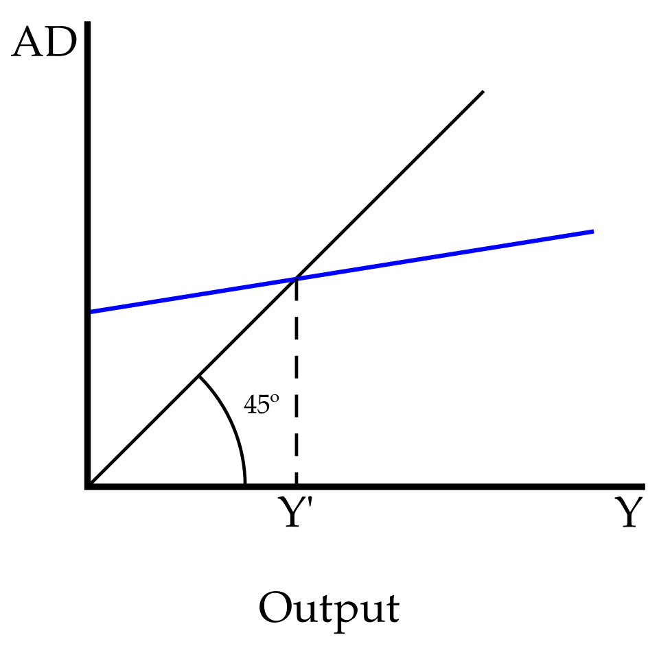 A 45° line (Y=PAE) intersecting a downward-sloping PAE curve at equilibrium Y. (Image: Tatenkopf, CC BY-SA 3.0, via Wikimedia Commons)
Why the 45° Line?
- The 45° line represents Y = PAE.
- Any point above the 45° line means firms are producing more than households plan to spend → unplanned inventory accumulation → firms cut production.
- Any point below the 45° line means households spend more than firms produce → unplanned inventory depletion → firms increase production.
- Equilibrium is where Y = PAE: no unplanned inventory changes.
Worked Example: Nepal’s PAE in 2023
Assume:
- C = 200 + 0.7Yd (where Yd = Y – T)
- T = 500 + 0.2Y (taxes)
- I = 200 (autonomous)
- G = 400
- X = 100, M = 50 + 0.1Y
Step 1: Express Yd in terms of Y Yd = Y – T = Y – (500 + 0.2Y) = 0.8Y – 500
Step 2: Write PAE PAE = C + I + G + (X – M) = (200 + 0.7*(0.8Y – 500)) + 200 + 400 + (100 – (50 + 0.1Y)) = 200 + 0.56Y – 350 + 200 + 400 + 50 – 0.1Y = (200 – 350 + 200 + 400 + 50) + (0.56Y – 0.1Y) = 500 + 0.46Y
Step 3: Set Y = PAE and solve Y = 500 + 0.46Y Y – 0.46Y = 500 0.54Y = 500 Equilibrium Y = Rs 925.93 billion
2. Consumption Function: How Households Spend
Consumption (C) depends on:
- Autonomous consumption (C₀): Spending even if income is zero (e.g., basic needs).
- Induced consumption: Spending that rises with income, governed by the Marginal Propensity to Consume (MPC).
Equation: C = C₀ + MPC × Yd Where Yd = Disposable Income = Y – T
Key Relationships
| Term | Definition | Example (Nepal) |
|---|---|---|
| MPC | ΔC/ΔYd (slope of consumption line) | If MPC = 0.7, a Rs 100 rise in Yd → Rs 70 more spending. |
| Marginal Propensity to Save (MPS) | 1 – MPC | If MPC = 0.7, MPS = 0.3. |
| Average Propensity to Consume (APC) | C/Yd | If C = 1000, Yd = 1200 → APC = 0.83. |
- X-axis: Yd (Rs 0 to 2000)
- Y-axis: C (Rs 0 to 1800)
- Slope = MPC = 0.7, intercept = C₀ = 200
- Shaded area = Savings (Yd – C).
Real World: eSewa and Consumption Smoothing
- eSewa’s "Save & Earn" feature lets users automatically save a fixed % of transactions (e.g., 10% of every Rs 1000 spent).
- This mimics autonomous savings (S₀).
- The remaining 90% is consumed → MPC ≈ 0.9 for that user.
- Why it matters: During COVID-19, eSewa users who saved via this feature had higher resilience when incomes dropped (lower MPC → higher MPS).
3. Savings and Investment: The Twin Engines
Savings Function
S = Yd – C Since C = C₀ + MPC × Yd, S = Yd – (C₀ + MPC × Yd) = (Yd – MPC × Yd) – C₀ = MPS × Yd – C₀
Key Point: Savings also has an autonomous component (–C₀) and an induced component (MPS × Yd).
- X-axis: Yd (Rs 0 to 2000)
- Y-axis: S (Rs –200 to 600)
- Slope = MPS = 0.3, intercept = –C₀ = –200
- Break-even point where S = 0 (if Yd = C₀/MPS = 200/0.3 ≈ Rs 666.67).
Investment vs. Savings
| Investment (I) | Savings (S) |
|---|---|
| Planned by firms (e.g., Daraz expanding warehouses). | Unplanned (e.g., households saving for a house). |
| Autonomous (doesn’t depend on Y). | Induced (depends on Yd). |
| Financed by savings in equilibrium. | Leakage from the circular flow. |
Worked Example: Daraz’s Warehouse Investment
- Daraz plans to build 5 new warehouses in Nepal (autonomous I = Rs 500 million).
- To fund this, Daraz borrows from banks (which rely on household savings).
- If MPS = 0.3, every Rs 1 of new savings supports Rs 3.33 of investment (via the multiplier).
4. The Multipliers: How Small Changes Have Big Effects
Multipliers show how an initial change in I, G, or T affects equilibrium Y.
Investment Multiplier (k)
Derivation:
- Initial I increases by ΔI.
- Households spend MPC × ΔI → firms earn this as new income.
- This income is partly saved (MPS × ΔI) and partly spent again (MPC × ΔI).
- The process repeats until savings "leak" the entire ΔI.
Formula: k = ΔY/ΔI = 1/MPS = 1/(1 – MPC)
Example: If MPC = 0.8 → MPS = 0.2 → k = 1/0.2 = 5. A Rs 100 million increase in I → Rs 500 million rise in Y.
Government Expenditure Multiplier (k_G)
Same logic as investment multiplier, but triggered by G: k_G = 1/MPS
Tax Multiplier (k_T)
Taxes reduce disposable income (Yd), which reduces C and thus Y. Formula: k_T = –MPC/MPS (Negative because higher taxes reduce Y.)
Example: If MPC = 0.7, MPS = 0.3 → k_T = –0.7/0.3 ≈ –2.33. A Rs 100 million tax hike → Rs 233 million drop in Y.
Foreign Trade Multiplier (k_XM)
Net exports (X – M) also affect Y. k_XM = 1/MPS (for exports) or –MPC/MPS (for imports).
Worked Example: Nepal’s Remittance Boom (2022)
- Remittances (X) rose by Rs 100 billion (autonomous increase in X).
- Assume MPS = 0.2 → k_XM = 1/0.2 = 5.
- Total impact on Y: Rs 100B × 5 = Rs 500 billion increase in GDP.
5. Autonomous vs. Induced Components
| Component | Definition | Example |
|---|---|---|
| Autonomous | Does not depend on Y or Yd. | Base consumption (C₀), investment (I), government spending (G). |
| Induced | Depends on Y or Yd. | C = C₀ + MPC × Yd, T = T₀ + MPT × Y. |
| Stabilizers | Automatic offsets to shocks (e.g., taxes rise when Y rises). | Progressive income tax, unemployment benefits. |
Mermaid Diagram: Circular Flow with Leakages and Injections
6. Policy Applications: How Nepal Uses Multipliers
Case 1: Post-Earthquake Reconstruction (2015)
- Problem: Earthquake destroyed Rs 800 billion in infrastructure.
- Policy: Government increased G by Rs 200 billion (autonomous).
- Effect:
- k_G = 1/MPS = 1/0.25 = 4 (assuming MPS = 0.25).
- Total GDP boost: Rs 200B × 4 = Rs 800 billion.
- But: Higher G also increased Y → higher T (if taxes are induced) → partial offset.
Case 2: Ncell’s 4G Expansion (2020)
- Investment: Ncell spent Rs 50 billion on 4G towers (I).
- Multiplier Effect:
- MPC = 0.6 → MPS = 0.4 → k = 1/0.4 = 2.5.
- Total impact: Rs 50B × 2.5 = Rs 125 billion rise in GDP.
- Induced effects:
- More jobs in construction → higher Y → higher C.
- Higher Y → higher tax revenue (T) for the government.
Case 3: Fiscal Stimulus During COVID-19
- Policy: Government cut taxes (T) by Rs 100 billion (autonomous).
- Tax Multiplier Effect:
- k_T = –MPC/MPS = –0.7/0.3 ≈ –2.33.
- Impact: Rs 100B tax cut → Rs 233 billion rise in Y.
- But: Higher Y → higher M (imports) → partial leakage.
## In the Real World
Khalti’s "Khalti Save" Feature
- Idea Used: Autonomous savings and MPC.
- How: Khalti allows users to auto-save a fixed % (e.g., 5%) of every transaction. This reduces their MPC for discretionary spending, increasing their MPS.
- Impact: Users with higher savings rates (lower MPC) contribute more to the financial system’s loanable funds, indirectly supporting investment (e.g., Daraz’s expansion).
NTC’s Fiber Expansion (2023)
- Idea Used: Investment multiplier and induced investment.
- How: NTC’s Rs 30 billion fiber rollout (I) created jobs in telecom infrastructure. The multiplier effect increased local incomes, boosting demand for NTC services (induced I via the accelerator effect).
- Real Numbers:
- Assume MPC = 0.7 → MPS = 0.3 → k = 3.33.
- Total GDP impact: Rs 30B × 3.33 ≈ Rs 100 billion.
Pathao’s Driver Incentives
- Idea Used: Government expenditure multiplier (via subsidies).
- How: Pathao partnered with local governments to subsidize driver training (part of G). This increased driver incomes (Y), which they spent on Pathao rides (induced C), boosting Pathao’s revenue.
- Example: A Rs 5 million subsidy for 1000 drivers → each driver’s Yd rises by Rs 5000.
- If MPC = 0.8 → each spends Rs 4000 on Pathao rides → Rs 4 million in induced revenue for Pathao.
## Exam Tip
Always derive multipliers from first principles:
- Start with Y = C + I + G + (X – M).
- Substitute C = C₀ + MPC × Yd and Yd = Y – T.
- Solve for Y to find equilibrium, then differentiate to get multipliers.
Memorize these formulas:
- Investment Multiplier: k = 1/MPS = 1/(1 – MPC).
- Tax Multiplier: k_T = –MPC/MPS.
- Government Multiplier: k_G = 1/MPS.
Watch for induced vs. autonomous:
- Autonomous terms (e.g., C₀, I, G) shift the entire PAE curve.
- Induced terms (e.g., MPC × Yd) change the slope of PAE.
Nepal-specific traps:
- Remittances (X) are autonomous (do not depend on Y).
- Imports (M) are induced (often written as M = M₀ + mY).
- Taxes (T) are often induced (T = T₀ + tY).
Graphical questions:
- Draw the Keynesian cross with:
- 45° line (Y = PAE).
- Downward-sloping PAE curve.
- Equilibrium where they intersect.
- For multipliers, show how a parallel shift in PAE (due to ΔI or ΔG) changes equilibrium Y.
- Draw the Keynesian cross with:
Numerical problems:
- Step 1: Write all structural equations (e.g., C, T, M).
- Step 2: Express Yd in terms of Y.
- Step 3: Write PAE = C + I + G + (X – M).
- Step 4: Substitute and solve Y = PAE.
- Step 5: For multipliers, differentiate or use the formulas above.
- Household consumption: 78%
- Government consumption: 12%
- Gross capital formation (investment): 25%
- Net exports: –5% (Source: NSB 2023)
Based on the TU BBA syllabus for Macro Economics (ECO204), unit 8.
Discussion
Loading…