Business StatisticsUnit 99 min read
ANOVA & Chi-Square: Hypothesis Testing for Group Differences & Categorical Data
Unit 9 of Business Statistics teaches how to compare means across multiple groups (ANOVA) and analyze categorical data relationships (Chi-Square), including test assumptions, calculations, and real-world applications in business decision-making.
Core Concepts: What ANOVA and Chi-Square Solve
1. Analysis of Variance (ANOVA): Testing Group Differences
ANOVA is used to determine whether three or more population means are equal. It compares the variability between groups to the variability within groups.
Key Idea: Partitioning Variance
ANOVA splits total variability into:
- Between-group variance (explained by group differences)
- Within-group variance (random error within groups)
If the between-group variance is significantly larger than the within-group variance, we reject the null hypothesis that all group means are equal.
Assumptions of ANOVA
mindmap
  root((ANOVA Assumptions))
    Normality["Data in each group is normally distributed"]
    Homogeneity["Variances (σ²) are equal across groups (Homogeneity of Variance)"]
    Independence["Observations are independent (no repeated measures)"]
    Randomness["Samples are randomly selected"]
Types of ANOVA
| Type | When to Use | Example |
|---|---|---|
| One-Way ANOVA | Compare means of one independent variable (e.g., treatment groups). | Testing if three different fertilizers affect crop yield. |
| Two-Way ANOVA | Compare means with two independent variables (e.g., treatment + location). | Testing if fertilizer and soil type affect crop yield. |
| Repeated-Measures ANOVA | Same subjects tested under multiple conditions (e.g., before/after training). | Comparing employee productivity before and after a training program. |
2. Chi-Square Test: Analyzing Categorical Data
Chi-Square tests whether observed frequencies differ from expected frequencies in categorical data.
Key Idea: Goodness-of-Fit vs. Test of Independence
| Test | Purpose | Example |
|---|---|---|
| Chi-Square Goodness-of-Fit | Check if observed data matches a hypothesized distribution. | Testing if a die is fair (each side appears 1/6th of the time). |
| Chi-Square Test of Independence | Check if two categorical variables are related. | Testing if education level (high/low) affects voting preference (Party A/B). |
Assumptions of Chi-Square
mindmap
  root((Chi-Square Assumptions))
    Independence["Observations are independent"]
    Expected["Expected frequency ≥5 in at least 80% of cells (for 2×2 tables)"]
    Categorical["Data is categorical (nominal/ordinal)"]
Step-by-Step Worked Examples
Example 1: One-Way ANOVA (Testing Fertilizer Effect on Crop Yield)
Scenario: A farmer tests three fertilizers (A, B, C) on 15 plots (5 per fertilizer). Yields (kg/plot) are:
| Fertilizer A | Fertilizer B | Fertilizer C |
|---|---|---|
| 45 | 50 | 40 |
| 48 | 52 | 42 |
| 42 | 48 | 38 |
| 50 | 55 | 45 |
| 47 | 53 | 41 |
Step 1: Calculate Group Means and Grand Mean
# Means per group
A_mean = (45+48+42+50+47)/5 = 46.4
B_mean = (50+52+48+55+53)/5 = 51.6
C_mean = (40+42+38+45+41)/5 = 41.2

# Grand mean
Grand_mean = (46.4*5 + 51.6*5 + 41.2*5)/15 = 46.4
Step 2: Calculate Sum of Squares (SS) Calculations:
- SSB = 5[(46.4-46.4)² + (51.6-46.4)² + (41.2-46.4)²] = 108.8
- SSW = Σ[(45-46.4)² + ... + (41-41.2)²] = 112.8
- SST = SSB + SSW = 221.6
Step 3: Compute Mean Squares (MS) and F-statistic
Step 4: Compare F to Critical Value
- Critical F (α=0.05, df1=2, df2=12) ≈ 3.89 (from F-table).
- Since 5.79 > 3.89, reject H₀. Fertilizers have a significant effect.
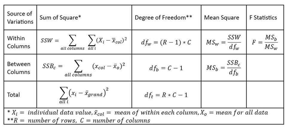 A labelled ANOVA table showing SSB, SSW, MS, and F-statistic. (Image: Luyan Li, CC BY 4.0, via Wikimedia Commons)
Example 2: Chi-Square Test of Independence (Education vs. Voting Preference)
Scenario: A survey of 200 voters shows:
| Party X | Party Y | Total | |
|---|---|---|---|
| High School | 30 | 50 | 80 |
| College | 40 | 20 | 60 |
| Graduate | 30 | 10 | 40 |
| Total | 100 | 80 | 180 |
Step 1: State Hypotheses
- H₀: Education level and voting preference are independent.
- H₁: They are dependent.
Step 2: Calculate Expected Frequencies For High School & Party X: Expected = (Row Total × Column Total) / Grand Total = (80 × 100) / 180 ≈ 44.44
Step 3: Compute Chi-Square Statistic
Step 4: Compare to Critical Value
- Critical Chi² (α=0.05, df=(2-1)(3-1)=2) ≈ 5.99.
- Since 14.11 > 5.99, reject H₀. Education level affects voting preference.
In the Real World
1. E-Sewa & Khalti: Testing User Experience Across Payment Methods
- ANOVA Application:
E-Sewa tests whether three payment methods (credit card, mobile wallet, bank transfer) affect transaction success rates.
- Groups: Payment methods (independent variable).
- Dependent Variable: Time taken to complete payment (in seconds).
- Business Use: If one method is significantly faster, E-Sewa can promote it to reduce dropout rates.
2. Daraz: Chi-Square Analysis of Customer Reviews by Product Category
- Chi-Square Application:
Daraz analyzes whether product category (electronics, fashion, groceries) is independent of review sentiment (positive/negative).
- Example: If electronics have more negative reviews than expected, Daraz can investigate quality control or adjust return policies.
3. NTC & Ncell: Comparing Network Performance Across Regions
- Two-Way ANOVA Application:
NTC tests if network speed varies by:
- Region (Kathmandu, Pokhara, Chitwan) (Factor 1).
- Time of Day (Morning, Evening, Night) (Factor 2).
- Business Use: If Pokhara has slower speeds at night, NTC can invest in infrastructure there.
4. NEPSE: Testing Stock Price Movements by Sector
- ANOVA Application:
NEPSE compares monthly returns of stocks in:
- Banking sector.
- Hydro sector.
- IT sector.
- Business Use: If one sector outperforms others significantly, investors can shift portfolios accordingly.
Common Mistakes & How to Avoid Them
| Mistake | Why It’s Wrong | Fix |
|---|---|---|
| Violating ANOVA assumptions | Non-normal data or unequal variances. | Use Kruskal-Wallis test (non-parametric alternative). |
| Incorrect degrees of freedom | Wrong df for F or Chi² tables. | ANOVA df: Between = k-1, Within = N-k. Chi² df: (rows-1)(cols-1). |
| Ignoring post-hoc tests | If ANOVA is significant, which groups differ? | Use Tukey’s HSD or Scheffé test. |
| Misinterpreting Chi-Square | Saying "variables are related" when p > α. | Only reject H₀ if Chi² > critical value. |
Exam Tip
What Examiners Look For
Correct Hypothesis Formulation
- Always write H₀ and H₁ clearly (e.g., "All group means are equal" vs. "At least one differs").
- For Chi-Square: "Variables are independent" vs. "Variables are dependent."
Step-by-Step Calculations
- Show SSB, SSW, SST for ANOVA.
- For Chi-Square, list observed vs. expected and compute (O-E)²/E for each cell.
Decision Rule
- Compare calculated F/Chi² to critical value (or use p-value).
- State whether to reject H₀ and interpret in context.
Assumption Checks
- Mention if data meets normality, homogeneity of variance (Levene’s test), or expected frequency ≥5.
Post-Hoc Analysis (ANOVA Only)
- If ANOVA is significant, mention Tukey’s test (even if not calculated).
Quick Revision Checklist
- Can I partition variance into between/within groups?
- Do I know when to use ANOVA vs. t-test (ANOVA for ≥3 groups)?
- Can I compute expected frequencies for Chi-Square?
- Do I interpret p-values correctly (p < 0.05 → reject H₀)?
Final Note: ANOVA and Chi-Square are powerful tools for business decisions—from marketing strategies (Khalti promotions) to operational efficiency (NTC network upgrades). Master the calculations and assumptions, and you’ll ace the exam!
Based on the TU BBM syllabus for Business Statistics (STT201), unit 9.
Discussion
Loading…