Introduction To Operations ManagementUnit 1112 min read
Transportation & Assignment Models: Cost Minimization & Optimal Allocation
Unit 11 of Introduction To Operations Management covers transportation problems (minimizing distribution costs) and assignment models (optimal task allocation), including mathematical formulations, solution methods (Vogel’s Approximation, MODI), and real-world applications in logistics, scheduling, and resource allocat
TAKEAWAYS:
- Transportation problems solve how to ship goods from sources to destinations at minimal cost using linear programming.
- Assignment models match tasks to workers/machines to minimize total time/cost (e.g., assigning drivers to routes).
- Vogel’s Approximation and MODI are shortcuts to solve these problems without full linear programming.
- Degeneracy occurs when a basic feasible solution has fewer allocations than variables—use dummy rows/columns to fix it.
- Real-world uses: Daraz’s warehouse-to-customer routes, Ncell’s technician assignments, and NTC’s vehicle scheduling.
1. Transportation Problems: Definitions and Basics
Transportation problems arise when goods must be moved from sources (factories, warehouses) to destinations (stores, customers) at the lowest possible cost. Key terms:
- Supply (S): Maximum units available at each source.
- Demand (D): Required units at each destination.
- Cost (C): Per-unit transportation cost from source i to destination j.
- Balanced problem: Total supply = total demand (no dummy rows/columns needed).
- Unbalanced problem: Requires adding a dummy source/destination to balance it.
Mathematical Formulation
Minimize total cost: Subject to:
Example: GC Manufacturing’s Distribution Problem
Given:
| Source \ Destination | A (P) | B (Q) | C (R) | Supply |
|---|---|---|---|---|
| P (5 units) | 5 | 10 | 3 | 5 |
| Q (20 units) | 10 | 3 | 20 | 20 |
| R (5 units) | 8 | 10 | 1 | 5 |
| Demand | 10 | 20 | 10 | 40 |
Step 1: Check balance Total supply = 5 + 20 + 5 = 30 units Total demand = 10 + 20 + 10 = 30 units → Balanced problem (no dummy needed).
Step 2: Initial Feasible Solution (Northwest Corner Rule) Start at the top-left cell (P→A) and allocate as much as possible:
- Allocate min(5, 10) = 5 to P→A. Update:
- P’s supply: 0, A’s demand: 5.
- Move right to P→B: min(0, 20) = 0 (skip).
- Move down to Q→B: min(20, 20) = 20 to Q→B. Update:
- Q’s supply: 0, B’s demand: 0.
- Move right to Q→C: min(0, 10) = 0 (skip).
- Move down to R→C: min(5, 10) = 5 to R→C. Update:
- R’s supply: 0, C’s demand: 5.
- Remaining demand for A: 5 → allocate to R→A: 5 (but R’s supply is exhausted). Issue: Demand for A is still 5 unmet. Solution: Use Vogel’s Approximation for a better initial solution.
flowchart TD
    A["Start: P→A (5)"] --> B["Update: P exhausted, A demand=5"]
    B --> C["Move right: P→B (0) → skip"]
    C --> D["Move down: Q→B (20)"]
    D --> E["Update: Q exhausted, B demand=0"]
    E --> F["Move right: Q→C (0) → skip"]
    F --> G["Move down: R→C (5)"]
    G --> H["Remaining A demand=5 → R→A (5)"]
Vogel’s Approximation Method (VAM)
Steps:
- For each row and column, calculate the penalty = difference between the two smallest costs in that row/column.
- Select the row/column with the highest penalty and allocate as much as possible to the lowest-cost cell in that row/column.
- Repeat until all supplies/demands are met.
Applying VAM to GC Manufacturing:
| Step | Row/Col | Costs | Penalties (Row/Col) | Allocation |
|---|---|---|---|---|
| 1 | Row P | 5, 10, 3 | (10-3)=7 | P→C (3) |
| 2 | Col C | 3, 20, 1 | (20-1)=19 (highest) | R→C (2) |
| 3 | Row R | 8, 10, 1 | (10-1)=9 | R→A (5) |
| 4 | Col A | 5, 8 | (8-5)=3 | Q→A (5) |
| 5 | Row Q | 10, 3, 20 | (10-3)=7 | Q→B (15) |
Final Allocation:
| Source | A (P) | B (Q) | C (R) | Supply |
|---|---|---|---|---|
| P | 0 | 0 | 3 | 5 |
| Q | 5 | 15 | 0 | 20 |
| R | 5 | 0 | 2 | 5 |
| Total Cost = (0×5) + (0×10) + (3×3) + (5×10) + (15×3) + (0×20) + (5×8) + (0×10) + (2×1) = 15 + 50 + 45 + 40 + 2 = 152 Rs. |
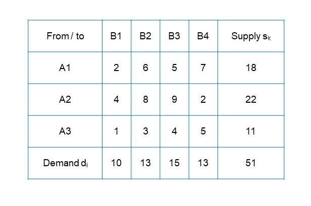 A labelled table showing supply, demand, and cost cells for GC Manufacturing’s problem. (Image: RVahrenkamp, CC BY-SA 4.0, via Wikimedia Commons)
2. Assignment Problems: Definitions and Basics
Assignment problems allocate tasks to workers/machines (or vice versa) to minimize total time/cost. Key terms:
- Jobs (J): Tasks to be assigned (e.g., routes, projects).
- Workers (W): Agents performing the tasks (e.g., drivers, technicians).
- Cost Matrix: Time/cost of assigning worker i to job j (denoted ).
- Objective: Assign each job to exactly one worker (and vice versa) to minimize total cost.
Mathematical Formulation
Minimize: Subject to:
Example: Worker Assignment at Ncell
Given: 4 workers (W1-W4) and 4 jobs (J1-J4) with the following cost matrix (time in hours):
| Worker \ Job | J1 (I1) | J2 (I2) | J3 (I3) | J4 (I4) |
|---|---|---|---|---|
| W1 | 2 | 3 | 0 | 1 |
| W2 | 1 | 2 | 1 | 3 |
| W3 | 4 | 2 | 3 | 2 |
| W4 | 3 | 1 | 2 | 4 |
Step 1: Hungarian Method (Step-by-Step)
Subtract row minima from each row:
- Row 1: min=0 → [2,3,0,1] → [2,3,0,1]
- Row 2: min=1 → [1,2,1,3] → [0,1,0,2]
- Row 3: min=2 → [4,2,3,2] → [2,0,1,0]
- Row 4: min=1 → [3,1,2,4] → [2,0,1,3]
Subtract column minima from each column:
- Col 1: min=0 → [2,0,2,2] → [2,0,2,2]
- Col 2: min=0 → [3,1,0,0] → [3,1,0,0]
- Col 3: min=0 → [0,0,1,1] → [0,0,1,1]
- Col 4: min=0 → [1,2,0,3] → [1,2,0,3]
Draw lines to cover all zeros with the fewest lines:
- Zeros at (W1,J3), (W2,J1), (W3,J4), (W4,J2).
- Optimal assignment: W1→J3, W2→J1, W3→J4, W4→J2.
Total Cost = 0 + 1 + 2 + 1 = 4 hours.
flowchart TD
    A["Step 1: Subtract row minima"] --> B["Step 2: Subtract column minima"]
    B --> C["Step 3: Cover zeros with min lines"]
    C --> D["Optimal Assignment:\nW1→J3, W2→J1, W3→J4, W4→J2"]
3. Comparison: Transportation vs. Assignment Problems
| Feature | Transportation Problem | Assignment Problem |
|---|---|---|
| Objective | Minimize shipping cost | Minimize total time/cost of task allocation |
| Variables | : units shipped from i to j | : binary (0/1) assignment |
| Constraints | Supply = Demand (balanced) | Each job/worker assigned exactly once |
| Solution Methods | Northwest Corner, VAM, MODI, Simplex | Hungarian Method, Linear Programming |
| Example | Daraz’s warehouse-to-customer routes | Ncell’s technician-to-repair-job assignments |
4. Real-World Applications
In the Real World
Daraz (Nepal’s Amazon)
- Transportation Problem: Daraz uses Vogel’s Approximation to optimize delivery routes from its warehouses in Kathmandu, Pokhara, and Biratnagar to customers across Nepal. For example, if Daraz has 3 warehouses (supply: 1000, 1500, 500 units) and 4 regions (demand: 800, 1200, 600, 400 units), it solves the problem to minimize fuel costs and delivery time.
- Assignment Problem: Daraz assigns delivery personnel to specific routes based on proximity and vehicle capacity. If a driver can cover 3 routes in a day, the assignment model ensures the most efficient pairing.
Ncell (Telecom Company)
- Assignment Problem: Ncell uses the Hungarian Method to assign technicians to repair jobs. For instance, if 4 technicians (W1-W4) need to fix 4 faulty towers (J1-J4) with varying travel times, the algorithm assigns W2 to J1 (1 hour) instead of W1 (2 hours), saving time and reducing costs.
NTC (Nepal’s Bus Company)
- Transportation Problem: NTC schedules buses from depots (e.g., Kathmandu, Pokhara) to routes (e.g., Kathmandu-Lalitpur, Pokhara-Chitwan) to minimize fuel and driver wages. If Depot A has 20 buses and Route 1 needs 15, the model ensures the cheapest allocation.
5. Solving Unbalanced Problems
If total supply ≠ total demand, add a dummy source/destination with:
- Zero cost for the dummy.
- Supply = excess demand (if supply > demand) or demand = excess supply (if demand > supply).
Example: Unbalanced Transportation Problem
Given:
| Source \ Destination | A | B | Supply |
|---|---|---|---|
| P | 4 | 2 | 10 |
| Q | 3 | 5 | 15 |
| Demand | 12 | 8 | 20 |
Solution:
- Total supply = 25, total demand = 20 → Add dummy destination D with demand = 5.
- New cost matrix: Add a column for D with all costs = 0.
| Source \ Destination | A | B | D | Supply |
|---|---|---|---|---|
| P | 4 | 2 | 0 | 10 |
| Q | 3 | 5 | 0 | 15 |
| Demand | 12 | 8 | 5 | 25 |
Apply VAM:
- Allocate P→B (8), Q→A (12), P→A (4), Q→D (5).
- Total Cost = (4×4) + (8×2) + (12×3) + (5×0) = 16 + 16 + 36 = 68 Rs.
6. Degeneracy in Transportation Problems
Degeneracy occurs when a basic feasible solution has fewer allocations than (where = sources, = destinations). This happens when a row/column has zero allocations.
Fixing Degeneracy
- Add a dummy allocation of 0 to a cell in the row/column with zero allocations.
- Use the MODI method to adjust the solution.
Example: Degenerate Solution
Initial Allocation:
| Source \ Destination | A | B | Supply |
|---|---|---|---|
| P | 5 | 0 | 5 |
| Q | 0 | 5 | 5 |
| Demand | 5 | 5 | 10 |
Issue: Row Q has only one allocation (Q→B), but . Solution: Add a dummy allocation of 0 to Q→A.
7. MODI (Modified Distribution Method)
MODI is used to test optimality of a transportation solution and improve it if needed.
Steps:
- Calculate (row factors) and (column factors) such that: for allocated cells.
- Check optimality: For unallocated cells, calculate .
- If all values ≥ 0 → optimal.
- If any value < 0 → not optimal; allocate to the most negative cell and re-optimize.
Example: Applying MODI
Given Allocation:
| Source \ Destination | A (u) | B (v) | Supply |
|---|---|---|---|
| P (u=0) | 5 (4) | 0 | 5 |
| **Q (u=?) ** | 0 | 5 (5) | 5 |
| Demand | 5 | 5 | 10 |
**Step 1: Assign , , . **Step 2: For Q→A (unallocated), , . From Q→B: → . Now, . Conclusion: Solution is optimal.
Exam Tip
- Always check balance: If supply ≠ demand, add a dummy row/column with zero costs.
- VAM > Northwest Corner: Vogel’s Approximation gives a better initial solution; prefer it in exams.
- Degeneracy handling: Add a dummy allocation of 0 if a row/column has no allocations.
- MODI for optimality: Use it to verify if your solution is optimal or needs adjustment.
- Assignment problems: The Hungarian Method is your best friend—memorize the row/column subtraction steps.
- Real-world tie-ins: Relate problems to Daraz’s logistics, Ncell’s technician assignments, or NTC’s bus scheduling in your answers.
Based on the TU BBM syllabus for Introduction To Operations Management (OPR311), unit 11.
Discussion
Loading…