Business StatisticsUnit 1010 min read
Cost and Production Analysis: Production Functions, Cost Curves, and Optimization
Unit 10 of Business Statistics: This note covers the relationship between inputs and outputs, the law of variable proportions, isoquants, isocosts, and the detailed analysis of short-run and long-run cost behaviors.
Key points
- Production functions describe the technical relationship between inputs (labor, capital) and the resulting output.
- The Law of Variable Proportions explains why marginal productivity eventually declines as more of a variable input is added to a fixed input.
- Optimal input combination is achieved where the isoquant curve is tangent to the isocost line.
- Total Cost is the sum of Fixed Costs (independent of output) and Variable Costs (dependent on output).
- A firm should shut down in the short run if the price falls below the Average Variable Cost (AVC).
Production Analysis
Production is the process of transforming inputs (factors of production) into outputs (goods and services). In business statistics and economics, we use a Production Function to express this relationship mathematically.
The Production Function
A production function shows the maximum amount of output that can be produced with a given set of inputs over a specific period. Where:
- : Quantity of output
- : Labor
- : Capital
- : Land
- : Entrepreneurship
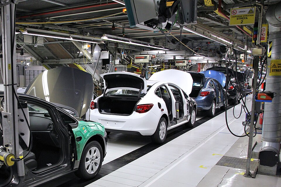 A typical production process showing inputs (raw materials, labor) being transformed into finished goods. (Image: Marek Ślusarczyk (Tupungato) Photo portfolio, CC BY 3.0, via Wikimedia Commons)
Short Run vs. Long Run
In production analysis, "short run" and "long run" are not fixed time periods (like a month or a year) but are defined by the flexibility of inputs.
The Law of Variable Proportions (Short Run)
This law states that as we increase the quantity of only one variable input (labor) while keeping other inputs (capital) fixed, the total product initially increases at an increasing rate, then at a decreasing rate, and eventually declines.
Key Terms:
- Total Product (TP): Total volume of goods produced.
- Average Product (AP): Output per unit of variable input.
- Marginal Product (MP): The additional output produced by adding one more unit of variable input.
The Three Stages of Production
- Stage I (Increasing Returns): MP increases and AP increases. The fixed factor is under-utilized.
- Stage II (Diminishing Returns): MP decreases but remains positive. AP also starts to fall. This is the rational stage where a firm prefers to operate.
- Stage III (Negative Returns): MP becomes negative, and TP starts to decline. Adding more labor actually hinders production (crowding).
Worked Example 1: Production at a Kathmandu Garment Factory Suppose a factory producing Pathao delivery bags has one sewing machine (fixed capital) and adds laborers.
| Labor (L) | Total Product (TP) | Marginal Product (MP) | Average Product (AP) |
|---|---|---|---|
| 0 | 0 | - | - |
| 1 | 10 | 10 | 10.0 |
| 2 | 25 | 15 | 12.5 |
| 3 | 45 | 20 | 15.0 |
| 4 | 60 | 15 | 15.0 |
| 5 | 70 | 10 | 14.0 |
| 6 | 75 | 5 | 12.5 |
| 7 | 75 | 0 | 10.7 |
| 8 | 70 | -5 | 8.75 |
Analysis:
- Stage I: From to . MP is rising; AP is rising.
- Stage II: From to . MP is falling but positive. TP reaches its maximum at .
- Stage III: From onwards. MP is negative; TP falls.
Isoquants and Isocosts (Long Run)
In the long run, a firm can vary both labor () and capital ().
Isoquant Curve
An isoquant is a curve showing all possible combinations of two inputs that yield the same level of output. It is similar to an indifference curve in consumer theory.
- Properties: Slopes downward, convex to the origin, and two isoquants never intersect.
Isocost Line
An isocost line shows all combinations of labor and capital that a firm can purchase with a given total budget. The equation is: Where:
- : Total Cost
- : Wage rate (cost of labor)
- : Rental rate (cost of capital)
Worked Example 2: Deriving the Isocost Line A furniture shop in Pokhara has a budget of Rs. 4,000. The wage rate () is Rs. 200 and the rental rate of capital () is Rs. 400.
- If all budget is spent on Labor:
- If all budget is spent on Capital:
Optimal Employment: The firm achieves the most efficient production when the Isoquant is tangent to the Isocost line. At this point, the ratio of marginal products equals the ratio of input prices:
Cost Analysis
Cost refers to the expenditure incurred by a firm to produce a commodity.
Short-Run Cost Concepts
- Total Fixed Cost (TFC): Costs that do not change with output (e.g., rent, permanent staff salary).
- Total Variable Cost (TVC): Costs that change directly with output (e.g., raw materials, electricity).
- Total Cost (TC): The sum of TFC and TVC.
- Average Fixed Cost (AFC): Fixed cost per unit. . It continuously declines as output increases.
- Average Variable Cost (AVC): Variable cost per unit. .
- Average Total Cost (AC): Total cost per unit. .
- Marginal Cost (MC): The change in total cost resulting from producing one additional unit.
Worked Example 3: Cost Schedule Analysis Consider the following data for a small bakery:
| Q | TFC | TVC | TC | AFC | AVC | AC | MC |
|---|---|---|---|---|---|---|---|
| 0 | 100 | 0 | 100 | - | - | - | - |
| 1 | 100 | 20 | 120 | 100 | 20 | 120 | 20 |
| 2 | 100 | 35 | 135 | 50 | 17.5 | 67.5 | 15 |
| 3 | 100 | 55 | 155 | 33.3 | 18.3 | 51.7 | 20 |
| 4 | 100 | 80 | 180 | 25 | 20 | 45 | 25 |
| 5 | 100 | 110 | 210 | 20 | 22 | 42 | 30 |
| 6 | 100 | 150 | 250 | 16.7 | 25 | 41.7 | 40 |
| 7 | 100 | 200 | 300 | 14.3 | 28.6 | 42.9 | 50 |
Observations:
- TFC remains constant at 100.
- AFC declines as output increases (the "spreading overhead" effect).
- AC and AVC are U-shaped due to the Law of Variable Proportions.
- MC cuts both AVC and AC at their minimum points.
The Shut-Down Decision
A firm must decide whether to continue operating or shut down in the short run when facing losses.
| Condition | Decision | Reason |
|---|---|---|
| Continue (Profit) | Firm covers all costs and earns profit. | |
| Continue (Loss) | Firm cannot cover TFC, but covers all TVC and some TFC. Loss is less than TFC. | |
| Shut Down | Firm cannot even cover its daily operating costs (TVC). Loss is greater than TFC. |
Worked Example 4: Shut-down Analysis A firm has:
- Average Revenue (Price) = Rs. 200
- Average Cost (AC) = Rs. 220
- Average Variable Cost (AVC) = Rs. 175
Calculation:
- Since , the firm is suffering a loss of Rs. 20 per unit.
- However, . Conclusion: The firm should stay in business in the short run. By continuing, it covers all its variable costs and contributes per unit toward its fixed costs. If it shuts down, it loses the entire TFC.
In the real world
- Daraz Warehouse Management: Daraz uses the Law of Variable Proportions when hiring seasonal staff during "11.11" sales. Initially, adding more sorters to a fixed number of conveyor belts increases efficiency (Stage I). However, if they hire too many people for the same space, workers get in each other's way, and productivity per person drops (Stage II and III).
- Ncell/NTC Infrastructure: For telecom companies, the towers and fiber-optic cables are Total Fixed Costs (TFC). Whether they have 1,000 or 1,000,000 users in a specific area, the tower cost remains the same. The cost of data packets and customer support is the Total Variable Cost (TVC).
- Commercial Banks (Loan Processing): A bank's loan department has a fixed cost (office rent, software licenses). As they process more loans, the Average Fixed Cost (AFC) per loan decreases, which is why banks prefer high volumes of transactions to lower their unit costs.
Exam tip
- The "Three Stages" Question: This is a favorite for 10-mark questions. Always draw the TP, MP, and AP graph. Clearly label the points where MP=0 (Max TP) and where MP cuts AP (Max AP).
- Shut-down Logic: If a numerical question asks whether a firm should shut down, don't just look at the profit/loss. Compare Price specifically with AVC. If , the answer is "Stay in business."
- Isocost/Isoquant: When asked to "derive" the isocost line, always calculate the X and Y intercepts (Total Budget / Wage and Total Budget / Rent) before drawing the straight line.
- Cost Relationships: Remember that MC always intersects AC and AVC at their lowest points. If your graph shows MC crossing AC while AC is still falling, it is technically incorrect.
Based on the TU BBS syllabus for Business Statistics (MGT207), unit 10.
Discussion
Loading…