Mathematical Methods in Economics: Functions, Elasticity & Optimization

TAKEAWAYS

• Functions in economics are mathematical models (linear, quadratic, exponential) that describe relationships like demand ($Q_d=a-bP$), supply ($Q_s=c+dP$), or cost ($TC=FC+VC$).
• Elasticity measures responsiveness: price elasticity of demand (PED) = %ΔQ/%ΔP (if |PED| > 1, demand is elastic; if < 1, inelastic). Income elasticity shows how demand changes with income.
• Optimization uses calculus (marginal analysis) to find profit-maximizing output ($MR=MC$) or cost-minimizing input combinations.
• Arc elasticity (for percentage changes over ranges) is calculated as: $$E=\frac{\Delta Q/\text{Average }Q}{\Delta P/\text{Average }P}$$ and is used for policy analysis (e.g., tax impact on supply).
• Real-world ties: Daraz uses demand functions to set dynamic pricing; Nabil Bank calculates loan interest via exponential growth models; NTC optimizes route costs with linear programming.
• Exam focus: Derive functions from tables, graph equilibria, compute elasticities, and interpret economic implications (e.g., "If PED = 0.5, a 10% price cut increases revenue by 5%").

1. Mathematical Functions in Economics

Economic relationships are often modeled using mathematical functions that relate variables like price ($P$), quantity ($Q$), cost ($C$), or income ($Y$). These functions can be linear, nonlinear, or exponential, depending on the context.

Key Function Types

Worked Example 1: Deriving Demand and Supply Functions

Problem: Given the following demand and supply schedules, derive the linear equations $Q_d=a-bP$ and $Q_s=c+dP$.

Solution:

1. Demand Function:

   • Use two points: $(P=10,Q_d=60)$ and $(P=50,Q_d=0)$.
   • Slope ($b$) = $\frac{\Delta Q_d}{\Delta P}=\frac{0-60}{50-10}=-2$.
   • Intercept ($a$): $0=a-2(50)\Rightarrow a=100$.
   • Equation: $Q_d=100-2P$.

2. Supply Function:

   • Use $(P=10,Q_s=10)$ and $(P=50,Q_s=50)$.
   • Slope ($d$) = $\frac{50-10}{50-10}=1$.
   • Intercept ($c$): $10=c+1(10)\Rightarrow c=0$.
   • Equation: $Q_s=P$.

Interpretation:

• Equilibrium: Where $Q_d=Q_s$: $100-2P=P\Rightarrow 100=3P\Rightarrow P=33.33$, $Q=33.33$.
• Real-world tie: Daraz uses similar demand functions to adjust prices dynamically based on inventory and competitor actions.

2. Elasticity: Measuring Responsiveness

Elasticity quantifies how much one variable responds to changes in another. In economics, we focus on:

1. Price Elasticity of Demand (PED)
2. Income Elasticity of Demand (YED)
3. Price Elasticity of Supply (PES)

Formulas

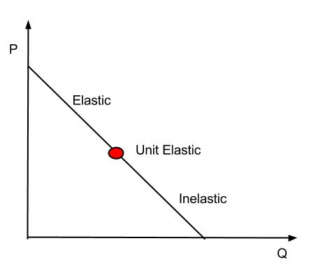Labels: Elastic (|PED| &gt; 1), Unit elastic (|PED| = 1), Inelastic (|PED| &lt; 1) (Image: Nber85, CC BY-SA 3.0, via Wikimedia Commons)

Worked Example 2: Calculating PED (Arc Method)

Problem: For Ncell, the demand for prepaid cards changes from 1000 units at Rs. 500 to 800 units at Rs. 600. Calculate the arc PED.

Solution:

1. Average Quantity: $\frac{1000+800}{2}=900$.
2. Average Price: $\frac{500+600}{2}=550$.
3. Change in Quantity: $800-1000=-200$.
4. Change in Price: $600-500=100$.
5. Arc PED: $$E_d=\frac{-200/900}{100/550}=\frac{-0.222}{0.182}=-1.22$$ Interpretation: $|E_d|=1.22>1$, so demand is elastic. A 1% increase in price reduces quantity demanded by 1.22%.

Real-world tie: Ncell uses elasticity to set promotional prices. If PED is elastic, lowering prices increases total revenue (e.g., "Buy 1 Get 1 Free" offers).

3. Optimization in Economics

Optimization uses calculus to find the best possible outcome (e.g., maximum profit, minimum cost). Key concepts:

• Marginal Analysis: Compare marginal benefits (MB) and marginal costs (MC).
• Profit Maximization: Occurs where $MR=MC$.
• Cost Minimization: Occurs where $M{P}_L/P_L=M{P}_K/P_K$ (for inputs).

Worked Example 3: Profit Maximization

Problem: A Daraz seller has the following revenue and cost functions:

• $TR=50Q-0.5Q^2$ (Total Revenue)
• $TC=100+10Q+0.1Q^2$ (Total Cost) Find the profit-maximizing quantity and maximum profit.

Solution:

1. Marginal Revenue (MR): Derivative of $TR$. $$MR=\frac{d(TR)}{dQ}=50-Q$$
2. Marginal Cost (MC): Derivative of $TC$. $$MC=\frac{d(TC)}{dQ}=10+0.2Q$$
3. Set $MR=MC$: $$50-Q=10+0.2Q\Rightarrow 40=1.2Q\Rightarrow Q=33.33$$
4. Maximum Profit: $$\pi =TR-TC=(50\times 33.33-0.5\times 33.33^2)-(100+10\times 33.33+0.1\times 33.33^2)$$ $$\pi =1666.5-555.5-100-333.3-111.1=566.6\text{ Rs.}$$

Real-world tie: Pathao optimizes driver routes using similar cost-revenue tradeoffs to minimize fuel costs while maximizing trip completions.

4. Applications in Real World

Example 1: Nabil Bank Loan Interest (Exponential Growth)

Nabil Bank calculates loan interest using the formula: $$A=P{\left(1+\frac{r}{n}\right)}^{nt}$$ where:

• $A$ = Amount to be repaid
• $P$ = Principal (loan amount)
• $r$ = Annual interest rate
• $n$ = Compounding frequency (e.g., 12 for monthly)
• $t$ = Time in years

Worked Example:

• Loan: Rs. 1,000,000 at 8% annual interest, compounded monthly, for 5 years.
• Calculation: $$A=1,000,000{\left(1+\frac{0.08}{12}\right)}^{12\times 5}=1,000,000\times 1.4859=1,485,900\text{ Rs.}$$
• Total Interest: Rs. 485,900.

Example 2: NTC Bus Route Optimization (Linear Programming)

NTC uses linear programming to minimize costs while meeting demand. For example:

• Objective: Minimize total cost $Z=50x+40y$ (where $x$ = buses on Route A, $y$ = buses on Route B).
• Constraints:
  • Demand: $x+y\ge 100$ (total buses)
  • Capacity: $2x+y\le 200$ (Route A has higher capacity)
  • Non-negativity: $x,y\ge 0$

Solution: Graph the constraints and find the feasible region. The optimal solution is at the intersection of $x+y=100$ and $2x+y=200$, giving $x=100$, $y=0$. Thus, NTC allocates all buses to Route A for minimum cost.

flowchart TD
    A["Constraints"] --> B["x + y ≥ 100"]
    A --> C["2x + y ≤ 200"]
    A --> D["x, y ≥ 0"]
    B --> E["Feasible Region"]
    C --> E
    E --> F["Optimal Point (100, 0)"]

Example 3: NEPSE Stock Price Elasticity

NEPSE tracks stock price elasticity to predict investor behavior. For example:

• If the price of a stock drops from Rs. 1000 to Rs. 900, and demand increases from 500 shares to 600 shares:
  • Arc PED: $$E_d=\frac{(600-500)/550}{(900-1000)/950}=\frac{100/550}{-100/950}=-1.73$$
  • Interpretation: $|E_d|=1.73>1$, so demand is elastic. Investors are highly responsive to price changes.

Exam Tip

1. Derive functions from tables: Always use two points to find slope and intercept.
2. Graph equilibria: Label axes, plot lines, and mark equilibrium points clearly.
3. Elasticity calculations: Use the arc method for percentage changes over ranges (common in exams).
4. Optimization: Remember $MR=MC$ for profit maximization and $M{P}_L/P_L=M{P}_K/P_K$ for cost minimization.
5. Real-world links: Connect theory to examples like:
   • Daraz: Demand functions for dynamic pricing.
   • Nabil Bank: Exponential growth for loan interest.
   • NTC: Linear programming for route optimization.
6. Common mistakes to avoid:
   • Forgetting absolute values for elasticity (PED can be negative, but we report $|E_d|$).
   • Misapplying arc vs. point elasticity formulas.
   • Ignoring units in economic interpretations (e.g., "Rs." or "units").

Summary Table: Key Formulas

Practice Questions

1. Given the supply schedule below, derive the supply function and calculate PES between Rs. 20 and Rs. 40.

   Price (Rs)	10	20	30	40
   Supply	50	100	150	200

2. A factory’s total cost is $TC=100+5Q+0.5Q^2$. Find the cost-minimizing output if the price of output is Rs. 15.

3. For the demand function $Q=100-2P$, calculate the PED at $P=20$ and interpret the result.

Note: Always show your working steps in exams, especially for derivations and calculations. Partial credit is often given for correct intermediate steps!