Taylor and Maclaurin Series – Definitions, Convergence, and Applications

Unit 10: Taylor and Maclaurin Series

1. Definition

A function $f$ that is infinitely differentiable at a point $a$ can be written as its Taylor series about $a$:

$$f(x)=\sum _{n=0}^{\infty }\frac{f^{(n)}(a)}{n!}(x-a{)}^n$$

where $f^{(n)}(a)$ denotes the $n$-th derivative of $f$ evaluated at $x=a$.
When $a=0$ the series is called a Maclaurin series:

$$f(x)=\sum _{n=0}^{\infty }\frac{f^{(n)}(0)}{n!}{x}^n$$

The partial sum

$$P_N(x)=\sum _{n=0}^N\frac{f^{(n)}(a)}{n!}(x-a{)}^n$$

is called the $N$-th degree Taylor polynomial.

2. Radius of Convergence

The series may converge only for $|x-a|<R$.
The radius $R$ is found by the ratio test:

$$R=\underset{n\to \infty }{\lim }\left|\frac{f^{(n)}(a)}{f^{(n+1)}(a)}\right|$$

If $R=\infty$, the series converges for all real $x$.
If $R=0$, the series is only valid at $x=a$.

3. Remainder (Error) Term

The difference between the function and its $N$-th Taylor polynomial is the remainder:

$$R_N(x)=f(x)-P_N(x)$$

In Lagrange form,

$$R_N(x)=\frac{f^{(N+1)}(\xi )}{(N+1)!}(x-a{)}^{N+1}$$

for some $\xi$ between $a$ and $x$.
This gives a bound on the truncation error:

$$|R_N(x)|\le \frac{{\max }_{\xi \in [a,x]}\left|f^{(N+1)}(\xi )\right|}{(N+1)!}|x-a{|}^{N+1}$$

4. Common Maclaurin Series

B${}_{2n}$ are Bernoulli numbers.

5. Worked Example – Maclaurin Series of $\sin x$

Compute the Maclaurin series up to $x^5$ and use it to approximate $\sin (0.1)$.

$$\sin x=x-\frac{x^3}{3!}+\frac{x^5}{5!}-\cdots$$

For $x=0.1$:

$$\sin (0.1)\approx 0.1-\frac{0.1^3}{6}+\frac{0.1^5}{120}=0.1-0.0001667+0.000000833=0.0998342$$

Exact value: $\sin (0.1)=0.0998334$.
Error $=8.6\times 10^{-7}$, well within the bound given by the remainder term.

6. Worked Example – Taylor Series of $f(x)=x^3-2x+4$ at $a=2$

Compute derivatives at $x=2$:

$$\begin{array}{rl}f(x)& =x^3-2x+4\\ f^{\prime }(x)& =3x^2-2\\ f^{\prime \prime }(x)& =6x\\ f^{\prime \prime \prime }(x)& =6\\ f^{(n)}(x)& =0(n\ge 4)\end{array}$$

Evaluate at $x=2$:

$$\begin{array}{rl}f(2)& =8-4+4=8\\ f^{\prime }(2)& =12-2=10\\ f^{\prime \prime }(2)& =12\\ f^{\prime \prime \prime }(2)& =6\end{array}$$

Taylor polynomial of degree 3:

$$P_3(x)=8+10(x-2)+\frac{12}{2!}(x-2{)}^2+\frac{6}{3!}(x-2{)}^3=8+10(x-2)+6(x-2{)}^2+1(x-2{)}^3$$

Since higher derivatives vanish, $P_3(x)=f(x)$ exactly.

7. Error Analysis – Lagrange Remainder

For $f(x)=e^x$, the $(N+1)$-th derivative is $e^x$.
Thus

$$|R_N(x)|\le \frac{e^{|x|}}{(N+1)!}|x{|}^{N+1}$$

For $x=0.5$ and $N=3$:

$$|R_3(0.5)|\le \frac{e^{0.5}}{4!}(0.5{)}^4\approx \frac{1.6487}{24}0.0625\approx 0.0043$$

Actual error using the first four terms is $0.0003$, well below the bound.

8. Comparison Table – Taylor vs. Maclaurin

9. Real‑World Applications

Worked Real‑World Example – Compound Interest
A student deposits $1000 in a bank offering 5 % annual interest compounded continuously. The amount after $t$ years is

$$A(t)=1000e^{0.05t}$$

For $t=1$ year, using the Maclaurin series up to $x^3$:

$$e^{0.05}\approx 1+0.05+\frac{0.05^2}{2}+\frac{0.05^3}{6}=1+0.05+0.00125+0.0000208=1.0512708$$

Thus $A(1)\approx 1000\times 1.0512708=1051.27$.
Exact value: $1000e^{0.05}=1051.271$. Error $<0.001$.

10. In the Real World

1. Google Search – The ranking algorithm uses Taylor expansions of logistic functions to approximate user relevance scores quickly.
2. WhatsApp – Signal processing of voice calls employs Maclaurin series of trigonometric functions for efficient Fourier transform approximations on mobile devices.
3. Daraz – Dynamic pricing models use exponential and logarithmic series to predict demand elasticity in real time.

11. Exam Tip

• Typical Questions

  1. Find the Maclaurin series of a given elementary function.
  2. Compute the Taylor series of a polynomial or rational function at a specified point.
  3. Determine the radius of convergence using the ratio test.
  4. Estimate the remainder using Lagrange’s form and provide an error bound.
  5. Apply a series to approximate a numerical value (e.g., $\sin 0.1$, $e^{0.5}$).

• Strategy

  1. Identify the function and its derivatives up to the required order.
  2. Write the general term and simplify.
  3. Use the ratio test for convergence.
  4. For error, find the maximum of the next derivative on the interval.
  5. Always check the domain of validity (radius of convergence).

• Common Mistakes

  • Forgetting the factorial in the denominator.
  • Using the wrong center for Taylor series.
  • Ignoring the sign alternation in $\sin$ and $\cos$ series.
  • Misapplying the remainder formula (using $x-a$ instead of $|x-a|$).

12. Visual Summary

flowchart TD
    "Start: f(x) smooth" --> "Compute f^(n)(a) for n=0,1,2,..."
    "Compute f^(n)(a)" --> "Form polynomial P_N(x)=Σ_{k=0}^N f^(k)(a)/k! (x-a)^k"
    "Form P_N(x)" --> "Check remainder R_N(x)=f(x)-P_N(x)"
    "Check remainder" --> "End"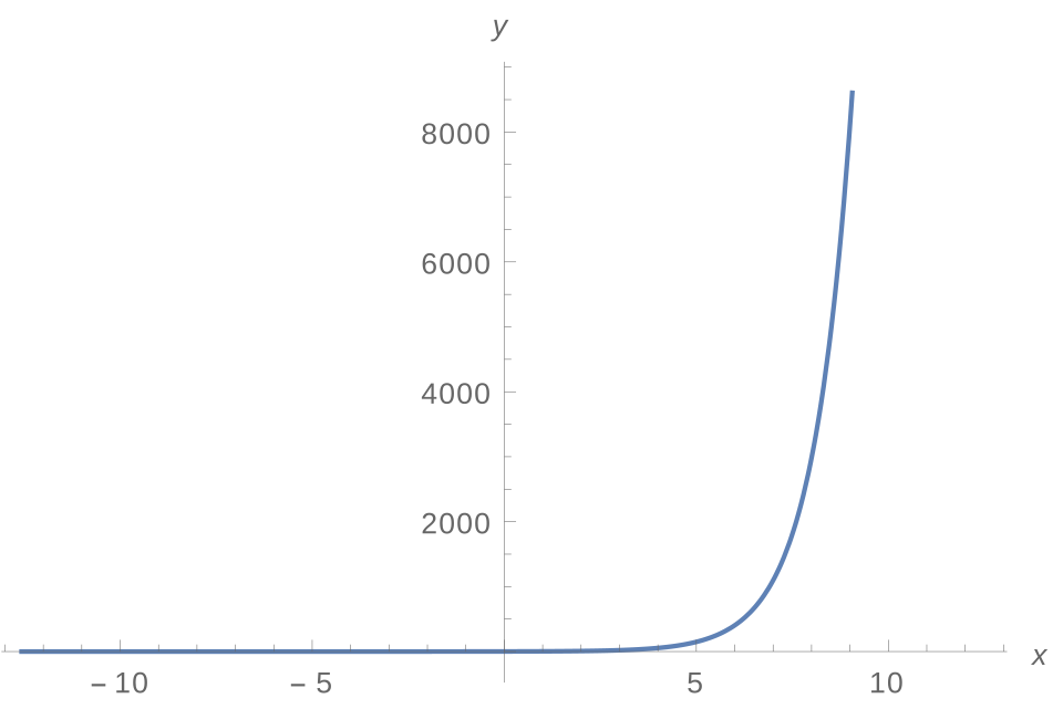

Graph of exponential function $e^x$ (Image: Derick Asamani, CC BY-SA 4.0, via Wikimedia Commons) 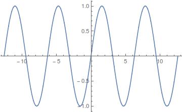Graph of sine function $\sin x$ (Image: Derick Asamani, CC BY-SA 4.0, via Wikimedia Commons)

END OF NOTE