Mathematics IIUnit 212 min read

Differential Calculus – Applications of Derivatives (Stationary points, optimisation, related rates, curve sketching)

Unit 2 of Mathematics II explains how derivatives are used to locate stationary and inflection points, solve optimisation and related‑rate problems, and sketch curves, with full worked examples and real‑world Nepalese applications.

Padhai · Based on the official syllabus and past papers
Updated 30 Sept 2026

Key points

Derivatives give the instantaneous rate of change and determine where a function increases, decreases or is flat.
Stationary points are classified by the first‑ and second‑derivative tests into maxima, minima or points of inflection.
Optimisation translates a word problem into a function, differentiates, and uses critical points to obtain the best (minimum or maximum) value.
Related‑rate problems connect several changing quantities through differentiation of a governing equation.
Curve sketching combines domain, intercepts, symmetry, monotonicity, concavity and asymptotes to produce a complete graph.

1. Why derivatives matter in applications

A derivative $f^{'} (x)$ measures how fast $y = f (x)$ changes with respect to $x$ . In engineering it is velocity, in economics it is marginal cost, and in everyday life it tells us when a quantity is rising or falling. All the application topics in this unit rely on the same logical chain:

Model the situation with a function $y = f (x)$ .
Differentiate to obtain $f^{'} (x)$ (and sometimes $f^{''} (x)$ ).
Set $f^{'} (x) = 0$ (or use a given rate) to locate critical points.
Classify using the first‑ or second‑derivative test.
Interpret the result in the original context (maximum profit, minimum distance, etc.).

2. Stationary points and the first‑derivative test

A stationary point occurs where the derivative is zero or undefined, i.e. $f^{'} (x) = 0$ (or $f^{'}$ does not exist) and the function is defined. The point may be a local maximum, local minimum, or a point of inflection.

2.1 First‑derivative test

Situation	Sign of $f^{'} (x)$ left of $c$	Sign of $f^{'} (x)$ right of $c$	Conclusion
$+$ → $-$	Positive	Negative	Local maximum at $x = c$
$-$ → $+$	Negative	Positive	Local minimum at $x = c$
$+$ → $+$ or $-$ → $-$	Same sign both sides	Same sign both sides	No extremum (possible plateau)

Worked example 1 – Finding stationary points

Find the stationary points of $f (x) = x^{3} - 6 x^{2} + 9 x + 2$ and classify them.

$f^{'} (x) = 3 x^{2} - 12 x + 9 = 3 (x^{2} - 4 x + 3) = 3 (x - 1) (x - 3)$

Set $f^{'} (x) = 0$ → $x = 1$ or $x = 3$ .

First‑derivative test

For $x < 1$ (e.g., $x = 0$ ): $f^{'} (0) = 9 > 0$ → increasing.
Between $1$ and $3$ (e.g., $x = 2$ ): $f^{'} (2) = 3 (1) (- 1) = - 3 < 0$ → decreasing.
For $x > 3$ (e.g., $x = 4$ ): $f^{'} (4) = 3 (3) (1) = 9 > 0$ → increasing.

Thus $x = 1$ is a local maximum, $x = 3$ a local minimum.

$f (1) f (3) = 1 - 6 + 9 + 2 = 6 = 27 - 54 + 27 + 2 = 2$

So the stationary points are $(1, 6)$ (max) and $(3, 2)$ (min).

3. Second‑derivative test and points of inflection

The second derivative $f^{''} (x)$ tells us about concavity:

$f^{''} (x) > 0$ → graph is concave upward (shaped like a cup).
$f^{''} (x) < 0$ → graph is concave downward (shaped like a cap).

A point of inflection occurs where concavity changes, i.e. $f^{''} (x) = 0$ (or undefined) and the sign of $f^{''}$ flips.

3.1 Second‑derivative test for stationary points

If $f^{'} (c) = 0$ and $f^{''} (c) \neq = 0$ :

$f^{''} (c) > 0$ → local minimum at $c$ .
$f^{''} (c) < 0$ → local maximum at $c$ .

If $f^{''} (c) = 0$ the test is inconclusive; revert to the first‑derivative test.

Worked example 2 – Inflection of a rational function

Determine the inflection points of $g (x) = \frac{x}{x ^{2} + 1}$ .

$g^{'} (x) g^{''} (x) = \frac{( x ^{2} + 1 ) - x ( 2 x )}{( x ^{2} + 1 ) ^{2}} = \frac{1 - x ^{2}}{( x ^{2} + 1 ) ^{2}} = \frac{- 2 x ( x ^{2} + 1 ) ^{2} - ( 1 - x ^{2} ) \cdot 2 ( x ^{2} + 1 ) ( 2 x )}{( x ^{2} + 1 ) ^{4}} = \frac{- 2 x ( x ^{2} + 1 ) - 4 x ( 1 - x ^{2} )}{( x ^{2} + 1 ) ^{3}} = \frac{- 2 x [ ( x ^{2} + 1 ) + 2 ( 1 - x ^{2} ) ]}{( x ^{2} + 1 ) ^{3}} = \frac{- 2 x [ - x ^{2} + 3 ]}{( x ^{2} + 1 ) ^{3}} = \frac{2 x ( x ^{2} - 3 )}{( x ^{2} + 1 ) ^{3}}$

Set $g^{''} (x) = 0$ → numerator $2 x (x^{2} - 3) = 0$ → $x = 0$ or $x = \pm 3$ .

Check sign change around each candidate:

Around $x = 0$ : pick $- 0.5$ (negative) → $g^{''} (- 0.5) < 0$ ; pick $0.5$ (positive) → $g^{''} (0.5) > 0$ . Sign changes → inflection at $x = 0$ .
Around $x = 3 \approx 1.732$ : pick $1.5$ (negative) → $g^{''} (1.5) < 0$ ; pick $2$ (positive) → $g^{''} (2) > 0$ . Sign changes → inflection at $x = 3$ .
Similarly for $- 3$ .

Thus three inflection points: $(0, 0)$ , $(3, \frac{3}{4})$ , $(- 3, \frac{- 3}{4})$ .

4. Optimisation problems

Optimisation asks for the maximum or minimum of a quantity subject to constraints. The standard steps are:

Define the quantity to optimise as a function $Q (x)$ .
Express any constraints to eliminate extra variables.
Differentiate $Q^{'} (x)$ and set to zero → critical points.
Use the second‑derivative test or endpoint evaluation to pick the best value.

4.1 Typical textbook pattern

“Find the dimensions of a rectangular box with a fixed surface area that yields the greatest volume.”

Worked example 3 – Minimum sum of squares (exam style)

Find two positive numbers whose sum is $20$ and whose sum of squares is minimum.

Let the numbers be $x$ and $20 - x$ . The sum of squares:

$S (x) = x^{2} + (20 - x)^{2} = x^{2} + 400 - 40 x + x^{2} = 2 x^{2} - 40 x + 400.$

Differentiate:

$S^{'} (x) = 4 x - 40.$

Set $S^{'} (x) = 0$ → $4 x - 40 = 0$ → $x = 10$ . Hence the other number is also $10$ .

Second derivative $S^{''} (x) = 4 > 0$ → minimum.

Result: The two numbers are $10$ and $10$ ; the minimum sum of squares is $1 0^{2} + 1 0^{2} = 200$ .

In a related‑rate problem several quantities change with time. The key is to differentiate the relationship with respect to time $t$ using the chain rule.

General recipe

Step	Action
1	Write an equation linking the variables (geometry, physics, etc.).
2	Differentiate implicitly with respect to $t$ .
3	Substitute known rates ( $\frac{d x}{d t}, \frac{d y}{d t}, \dots$ ).
4	Solve for the unknown rate.

Worked example 4 – Ladder sliding down a wall (classic)

A 5 m ladder leans against a vertical wall. The foot slides away at $1.2 m/s$ . Find the speed at which the top slides down when the foot is $3 m$ from the wall.

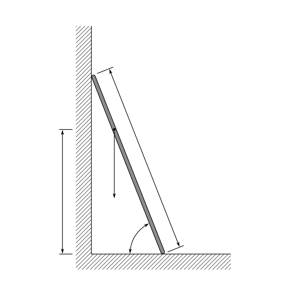ladder leaning against wall diagram Diagram of a ladder leaning against a wall (Image: Steven Baltakatei Sandoval, CC BY-SA 4.0, via Wikimedia Commons)

Let $x$ = distance of foot from wall, $y$ = height of top. By Pythagoras:

$x^{2} + y^{2} = 5^{2} = 25.$

Differentiate w.r.t. $t$ :

$2 x \frac{d x}{d t} + 2 y \frac{d y}{d t} = 0 ⟹ x \frac{d x}{d t} + y \frac{d y}{d t} = 0.$

Given $d x / d t = 1.2 m/s$ and $x = 3$ . Find $y$ from the original relation:

$y = 25 - 3^{2} = 16 = 4 m .$

Now solve for $d y / d t$ :

$3 (1.2) + 4 \frac{d y}{d t} = 0 ⟹ \frac{d y}{d t} = - \frac{3.6}{4} = - 0.9 m/s .$

The negative sign indicates the top is descending at $0.9 m/s$ .

6. Curve sketching – putting all pieces together

A complete sketch of a function $f (x)$ requires:

Domain and range.
Intercepts (x‑ and y‑).
Symmetry (even/odd).
Asymptotes (vertical/horizontal/oblique).
Critical points (where $f^{'} = 0$ or undefined).
Concavity (sign of $f^{''}$ ).
Inflection points (where concavity changes).

Worked example 5 – Sketch $h (x) = \frac{x ^{2}}{x ^{2} - 4}$

Feature	Computation
Domain	$x^{2} - 4 \neq = 0$ → $x \neq = \pm 2$ .
Intercepts	$h (0) = 0$ → y‑intercept at $(0, 0)$ . No x‑intercept except at 0.
Symmetry	Even (replace $x$ by $- x$ → same).
Vertical asymptotes	$x = \pm 2$ .
Horizontal asymptote	$x \to \pm \infty lim \frac{x ^{2}}{x ^{2} - 4} = 1$ → $y = 1$ .
First derivative	$h^{'} (x) = \frac{2 x ( x ^{2} - 4 ) - x ^{2} ( 2 x )}{( x ^{2} - 4 ) ^{2}} = \frac{- 8 x}{( x ^{2} - 4 ) ^{2}}$ .
Critical points	$h^{'} (x) = 0$ → $x = 0$ .
Second derivative	$h^{''} (x) = \frac{- 8 ( x ^{2} - 4 ) ^{2} + 16 x ^{2} ( x ^{2} - 4 )}{( x ^{2} - 4 ) ^{4}} = \frac{8 ( 3 x ^{2} - 4 )}{( x ^{2} - 4 ) ^{3}}$ .
Inflection	Set numerator $3 x^{2} - 4 = 0$ → $x = \pm \frac{2}{3}$ .

Behaviour summary

For $∣ x ∣ < 2$ : denominator negative → $h (x) < 0$ .
For $∣ x ∣ > 2$ : denominator positive → $h (x) > 0$ .
At $x = 0$ : local minimum $h (0) = 0$ .
Concave up for $∣ x ∣ > \frac{2}{3}$ ; concave down for $∣ x ∣ < \frac{2}{3}$ (inside each interval).

7. Comparison of tests for extrema

First‑derivative test works for any differentiable function, even when $f^{''} (c) = 0$ .
Second‑derivative test is quicker when $f^{''} (c) \neq = 0$ but fails at points of inflection or higher‑order flatness.
Endpoint analysis is essential for closed intervals (common in exam problems).

8. In the real world

Product / Service	Derivative idea used	How it is applied
eSewa & Khalti (digital wallets)	Rate of change of transaction volume → marginal cost analysis	The platforms monitor the derivative of daily transaction count to predict server load spikes and dynamically allocate cloud resources, ensuring smooth payment processing during festivals.
Daraz order queue	Optimisation of delivery routes (minimising total distance)	By modelling total travel distance $D (x)$ as a function of route parameters, Daraz uses the first‑derivative test to locate the route that gives the smallest $D$ , reducing fuel consumption and delivery time.
NEPSE (stock exchange)	Maximum profit point (price‑time curve)	Traders compute the derivative of a stock’s price curve to find where the slope changes from positive to negative, indicating a local maximum price – the optimal sell point.
Google Maps traffic flow	Related rates (changing traffic density)	When a road segment’s vehicle count $N (t)$ changes, Google differentiates the relationship $N = ρ \cdot L$ (density × length) to estimate the rate at which congestion builds, updating ETA in real time.
Bank loan interest	Minimising total interest (optimisation)	A bank designs loan repayment schedules $I (p) = \frac{p ^{2}}{( L - p )}$ where $p$ is the principal paid early. Differentiating gives the optimal early‑payment amount that minimises total interest for the borrower.

Real‑situated worked example

A Daraz seller wants to price a product to maximise revenue. Revenue $R (p) = p \cdot q (p)$ where demand $q (p) = 120 - 2 p$ (units per day). Find the price that yields maximum revenue.

$R (p) = p (120 - 2 p) = 120 p - 2 p^{2} .$

$R^{'} (p) = 120 - 4 p$ . Set to zero → $p = 30$  NRs.

Second derivative $R^{''} (p) = - 4 < 0$ → maximum.

Thus the seller should price the item at 30 NRs to achieve the highest daily revenue of $R (30) = 30 (120 - 60) = 1800$  NRs.

9. Common pitfalls and how to avoid them

Pitfall	Why it happens	Remedy
Forgetting to check endpoints on a closed interval	Focus only on critical points	Always list $f (a)$ and $f (b)$ before concluding.
Using the second‑derivative test when $f^{''} (c) = 0$	Assumes non‑zero curvature	Revert to the first‑derivative sign test.
Mixing up rates ( $d x / d t$ vs. $d x$ ) in related‑rate problems	Implicit differentiation can be skipped	Write the governing equation explicitly, then differentiate term‑by‑term.
Mis‑identifying the domain of a rational function	Overlooking denominator zeros	Factor denominator first, state restrictions clearly.
Ignoring units in optimisation (e.g., mixing meters and centimeters)	Leads to wrong numerical answer	Keep a consistent unit system throughout the problem.

10. Exam tip

The exam frequently asks you to “find the stationary points and determine their nature” or “solve an optimisation problem”.

Write a short checklist on your scrap paper:
- Compute $f^{'} (x)$ .
- Solve $f^{'} (x) = 0$ .
- Apply first‑derivative sign test or second‑derivative test.
- Evaluate endpoints if the interval is closed.
For optimisation, translate the word problem into a single‑variable function before differentiating. Eliminate extra variables using the given constraint.
Related‑rate questions: draw a quick diagram, label all known rates, differentiate, then substitute.
Time‑saving: if $f^{''} (c) \neq = 0$ you can skip the sign‑chart and directly state max/min.

Mark each step clearly; the examiner awards marks for the logical process even if the final arithmetic contains a small slip.

Based on the TU BCA syllabus for Mathematics II (CAMT154), unit 2.

Discussion

Loading…