Mathematics IIUnit 77 min read
Linear Programming: Simplex Method – Basics, Tableau, and Applications
Unit 7 of Mathematics II: This note covers linear programming fundamentals, simplex algorithm steps, tableau construction, pivot rules, duality, and real‑world applications such as resource allocation in eSewa and delivery routing in Pathao.
Key points
- Linear programming models optimization problems with linear objective and constraints.
- The simplex method iteratively moves along vertices of the feasible polytope using pivot operations.
- A tableau encodes the system; pivoting selects entering and leaving variables to improve the objective.
- Optimality is reached when all reduced costs are non‑positive (for maximization).
- Duality links primal and dual problems, providing bounds and sensitivity insights.
- Simplex is efficient for most practical problems but can suffer from cycling; modern variants and interior‑point methods address this.
1. What is Linear Programming?
Linear programming (LP) is a mathematical framework for optimizing a linear objective function subject to linear equality or inequality constraints.
- Decision variables represent quantities to be determined.
- Objective function is to be maximized or minimized.
- Constraints are linear inequalities or equalities of the form
- Non‑negativity is usually imposed.
The set of all feasible solutions is a convex polyhedron (feasible region). The optimum lies at a vertex (basic feasible solution).
2. Standard Form
For the simplex method we convert every LP to standard form:
where is an matrix, is an -vector, and is an -vector.
- Slack variables convert constraints into equalities: .
- Surplus + artificial variables handle constraints.
3. Tableau Representation
A simplex tableau is a compact tabular form that stores the coefficients of the constraints, the objective function, and the current basic variables.
| Basic | RHS | ||||
|---|---|---|---|---|---|
| 1 | 2 | 1 | 0 | 6 | |
| 4 | 3 | 0 | 1 | 6 | |
| -7 | -5 | 0 | 0 | 0 |
Table 1: Initial tableau for the example in Section 5.
The bottom row contains the reduced costs (coefficients of non‑basic variables in the objective).
4. Simplex Algorithm – Step‑by‑Step
- Identify entering variable: Choose a non‑basic variable with the most negative reduced cost (for maximization).
- Identify leaving variable: Compute the minimum ratio over all rows where .
- Pivot: Perform row operations to make the pivot element and all other entries in the pivot column .
- Update tableau: Repeat until all reduced costs are .
4.1 Worked Example
Problem
Maximize
subject to
Step 0 – Convert to Standard Form
Add slack variables :
Step 1 – Initial Tableau (Table 1 above).
Step 2 – Pivot Selection
- Reduced costs: (for ), (for ).
- Entering variable: (most negative).
- Ratios: (row 1), (row 2).
- Leaving variable: (smallest ratio).
Step 3 – Pivot on
After row operations:
| Basic | RHS | ||||
|---|---|---|---|---|---|
| 1 | 0.75 | 0 | 0.25 | 1.5 | |
| 0 | 1.25 | 1 | -0.25 | 4.5 | |
| 0 | 1.75 | 0 | 1.75 | 10.5 |
Step 4 – Check Optimality
Reduced costs: has (non‑negative), so the current solution is optimal.
Optimal Solution
.
5. Visualizing the Feasible Region
Figure 1: Feasible region and constraint lines for the worked example. The optimal vertex is at .
6. Pivot Rules and Variants
| Rule | Description | Pros | Cons |
|---|---|---|---|
| Bland’s Rule | Choose the smallest index variable to enter/leave. | Guarantees no cycling. | Can be slow. |
| Dantzig’s Rule | Choose variable with most negative reduced cost. | Fast convergence in practice. | May cycle (rare). |
| Steepest Edge | Choose variable that gives largest increase per unit cost. | Faster in high‑dimensional problems. | Requires extra computation. |
7. Duality
Every LP has a dual problem.
- Primal (P): maximize subject to .
- Dual (D): minimize subject to .
The Weak Duality Theorem states for any feasible .
The Strong Duality Theorem guarantees equality at optimality.
Duality provides bounds, sensitivity analysis, and economic interpretation (e.g., shadow prices).
8. Sensitivity Analysis
After solving an LP, we can ask:
- How does the optimal value change if changes?
- What is the allowable range for a coefficient before the basis changes?
These questions are answered by examining the shadow price (dual variable) and the reduced cost in the final tableau.
9. Advantages & Disadvantages
| Advantage | Disadvantage |
|---|---|
| Simple to implement. | Can cycle (rare). |
| Works well for medium‑size problems. | Not efficient for very large sparse systems. |
| Provides optimal solution and dual values. | Requires all data to be linear. |
| Easy to interpret solutions. | Sensitive to numerical errors in degenerate cases. |
10. Real‑World Applications
10.1 eSewa – Cash‑less Payments
- Problem: Allocate limited transaction bandwidth to maximize revenue.
- LP Idea: Objective = revenue per transaction; constraints = server capacity, transaction limits.
- Result: Optimal allocation of transaction slots to merchants.
10.2 Daraz – Order Fulfilment Queue
- Problem: Schedule pick‑up and delivery to minimize total delivery time.
- LP Idea: Variables = number of orders assigned to each courier; constraints = courier capacity, delivery windows.
- Result: Efficient routing and load balancing.
10.3 Pathao – Ride‑Sharing Pricing
- Problem: Set dynamic fares to maximize profit while keeping demand within driver supply.
- LP Idea: Objective = profit = fare × number of rides; constraints = driver availability, minimum service level.
- Result: Real‑time fare adjustments.
11. In the Real World
- Google Ads: Uses LP to allocate ad slots to maximize click‑through revenue under budget constraints.
- Ncell Network Planning: Optimizes tower placement and bandwidth allocation using LP models.
- NEPSE Trading: Portfolio optimization to maximize expected return subject to risk limits.
12. Exam Tip
- Know the tableau format: Be able to write the initial tableau quickly.
- Pivot selection: Practice identifying entering/leaving variables and performing row operations.
- Optimality check: Remember that for maximization all reduced costs must be .
- Duality: Be prepared to write the dual of a given primal problem.
- Sensitivity: Understand how to read shadow prices from the final tableau.
13. Real Pictures
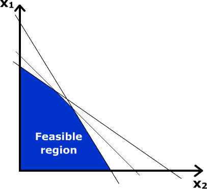 Feasible region of a two‑variable LP (Image: en:User:Jacj, Public domain, via Wikimedia Commons)
 Example of resource allocation in manufacturing (Image: Marek Ślusarczyk (Tupungato) Photo portfolio, CC BY 3.0, via Wikimedia Commons)
Based on the TU BCA syllabus for Mathematics II (CAMT154), unit 7.
Discussion
Loading…