Data Structures And AlgorithmsUnit 1216 min read
Algorithm Analysis: Big-O, Complexity, Divide & Conquer, Greedy, Dynamic
Unit 12 of Data Structures And Algorithms covers algorithmic complexity analysis using Big-O notation, time/space tradeoffs, divide-and-conquer strategies, greedy algorithms, and dynamic programming. It teaches how to classify algorithms by efficiency, compare their performance, and apply optimization techniques to rea
TAKEAWAYS:
- Big-O notation describes algorithmic efficiency by focusing on growth rate (e.g., , , ), ignoring constants and lower-order terms.
- Divide-and-conquer splits problems into smaller subproblems (e.g., merge sort, binary search), reducing complexity from to .
- Greedy algorithms make locally optimal choices (e.g., Dijkstra’s shortest path, Huffman coding) but may not always yield globally optimal solutions.
- Dynamic programming solves overlapping subproblems by storing intermediate results (e.g., Fibonacci sequence, knapsack problem) to avoid redundant calculations.
- Space-time tradeoffs exist: some algorithms use more memory (e.g., memoization) to save computation time.
- Amortized analysis explains why operations like
append()in dynamic arrays appear on average despite occasional resizing.
1. Why Analyze Algorithms?
Algorithms are the backbone of software efficiency. Without analysis, we cannot predict:
- How long a program will run for large inputs (e.g., sorting 1 million records).
- How much memory it will consume (e.g., storing a graph with 10,000 nodes).
- Whether it will scale for real-world use (e.g., handling 1000+ concurrent users in an app).
Example: A linear search () takes 1 second for 100 items. For 1 million items, it would take 10,000 seconds (~2.7 hours). A binary search () would take only 20 seconds for the same dataset.
2. Big-O Notation: The Language of Efficiency
Big-O describes the upper bound of an algorithm’s growth rate as input size increases. It ignores:
- Constants (e.g., → ).
- Lower-order terms (e.g., → ).
Common Complexity Classes
| Notation | Name | Example Algorithm | Growth Rate |
|---|---|---|---|
| Constant | Array indexing | Never grows | |
| Logarithmic | Binary search | Slow growth | |
| Linear | Linear search | Grows proportionally | |
| Linearithmic | Merge sort, quicksort | Balanced growth | |
| Quadratic | Bubble sort, insertion sort | Fast growth | |
| Exponential | Recursive Fibonacci | Explosive growth | |
| Factorial | Traveling Salesman (brute-force) | Catastrophic |
Visual: Growth Rates
Key Rules:
- Worst-case analysis: Big-O describes the slowest possible scenario.
- Asymptotic behavior: Focus on behavior as .
- Not exact runtime: It does not give seconds or milliseconds.
Example: For the algorithm:
def sum_array(arr):
    total = 0
    for num in arr:       # O(n)
        total += num
    for num in arr:       # O(n)
        total += num
    return total           # O(1)
The total complexity is .
3. In the Real World
Example 1: eSewa and Khalti (Payment Processing)
- Idea Used: Greedy Algorithm for Transaction Routing
- When you pay via eSewa/Khalti, the app must quickly route your transaction to the nearest bank or payment gateway.
- A greedy approach selects the closest available server (lowest latency) without reconsidering past choices, ensuring near-instant processing.
- Why it matters: If Khalti used a brute-force method (), processing 1000 transactions would take years.
Example 2: Daraz (Order Fulfillment Queue)
- Idea Used: Priority Queue (Greedy + Divide-and-Conquer)
- Daraz prioritizes orders based on urgency (e.g., "Same-day delivery") and distance from warehouse.
- A min-heap (priority queue) ensures the most urgent order is processed first ( insertion).
- Real-world impact: Without this, a customer ordering at 11:59 PM might get their package after someone who ordered at 12:01 AM.
Example 3: NTC (Network Routing with Dijkstra’s Algorithm)
- Idea Used: Shortest Path (Greedy + Dynamic Programming)
- The Nepal Telecommunications Company (NTC) uses Dijkstra’s algorithm to route internet traffic through the least congested paths.
- How it works:
- Start from the source node (e.g., Kathmandu).
- Greedily pick the cheapest path to each neighbor.
- Update distances dynamically as new data arrives.
- Result: Faster internet speeds and reduced costs.
Example 4: NEPSE (Stock Market Matching)
- Idea Used: Divide-and-Conquer for Order Matching
- When you buy/sell stocks on NEPSE, the system must match buy/sell orders in milliseconds.
- A divide-and-conquer approach splits orders into price buckets (e.g., ₹100–₹110) and matches them locally before merging results.
- Why it’s critical: A delay of even 1 second could cost traders millions.
Example 5: Pathao (Ride Matching with Hashing)
- Idea Used: Hash Tables for Rider-Driver Matching
- Pathao uses geohashing to group riders/drivers by location (e.g., "Kathmandu-3" → all users near Thapathali).
- When you request a ride, Pathao hashes your location to find the nearest driver in time.
- Without hashing: A linear search () would make ride requests take minutes instead of seconds.
4. Divide-and-Conquer: Breaking Problems into Smaller Pieces
Definition: An algorithm that:
- Divides a problem into smaller subproblems of the same type.
- Conquers each subproblem recursively.
- Combines the results to solve the original problem.
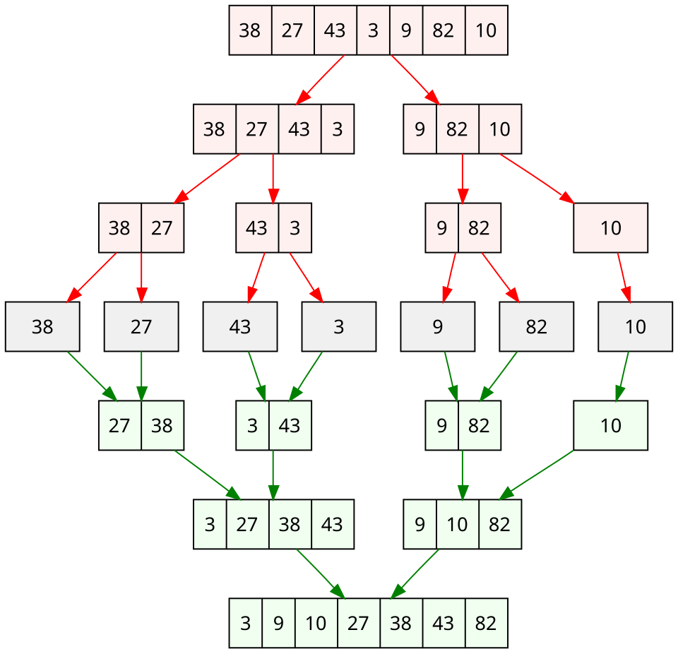 Merge sort: Divide, conquer, and combine phases (Image: VineetKumar at English Wikipedia, Public domain, via Wikimedia Commons)
Key Examples:
- Binary Search ()
- Divides a sorted array into halves until the target is found.
- Merge Sort ()
- Splits the array, sorts subarrays, and merges them.
- Strassen’s Matrix Multiplication
- Reduces matrix multiplication from to .
Algorithm: Binary Search
flowchart TD
    A["Start"] --> B["Set low=0, high=n-1"]
    B --> C{"Is low <= high?"}
    C -->|"Yes"| D["mid = (low + high)/2"]
    D --> E{"Is arr[mid] == target?"}
    E -->|"Yes"| F["Return mid"]
    E -->|"No"| G{"Is arr[mid] < target?"}
    G -->|"Yes"| H["low = mid + 1<br/>Go to C"]
    G -->|"No"| I["high = mid - 1<br/>Go to C"]
    C -->|"No"| J["Return -1 (Not found)"]
Code Implementation:
def binary_search(arr, target):
    low, high = 0, len(arr) - 1
    while low <= high:
        mid = (low + high) // 2
        if arr[mid] == target:
            return mid
        elif arr[mid] < target:
            low = mid + 1
        else:
            high = mid - 1
    return -1
Trace for arr = [1, 3, 5, 7, 9], target = 5:
| Step | low | high | mid | arr[mid] | Action |
|---|---|---|---|---|---|
| 1 | 0 | 4 | 2 | 5 | Found! Return 2 |
Real-World Trace: NTC Internet Routing
Suppose NTC has a sorted list of ISPs by latency (in ms):
[10, 20, 30, 40, 50, 60, 70, 80, 90, 100]
You want the fastest ISP under 40 ms.
- Step 1:
low=0,high=9,mid=4→arr[4]=50(too high) →high=3. - Step 2:
mid=1→arr[1]=20(valid) → select ISP 20 ms.
5. Greedy Algorithms: Making the Best Local Choice
Definition: An algorithm that makes the locally optimal choice at each step, hoping it leads to a globally optimal solution.
When to Use:
- Problems with optimal substructure (e.g., shortest path, Huffman coding).
- No need to reconsider past choices (e.g., coin change with fixed denominations).
When It Fails:
- If local choices conflict with global goals (e.g., activity selection with overlaps).
Example 1: Dijkstra’s Shortest Path (NTC Network Routing)
Problem: Find the shortest path from Kathmandu to Pokhara with the following graph (weights = latency in ms):
Algorithm Steps:
- Start at Kathmandu (
dist[K] = 0). - Pick the nearest unvisited node (greedy choice).
- Update distances to neighbors.
Trace:
| Step | Node | dist | Path | Action |
|---|---|---|---|---|
| 1 | K | 0 | - | Visit K, update B (20), L (30) |
| 2 | B | 20 | K→B | Visit B, update N (20+15=35) |
| 3 | L | 30 | K→L | Visit L, update N (min(35,30+25)=55) |
| 4 | N | 35 | K→B→N | Visit N, update P (35+10=45) |
| 5 | P | 45 | K→B→N→P | Done! |
Final Path: Kathmandu → Bhaktapur → Nepalgunj → Pokhara (45 ms).
Why Greedy Works Here:
- Each step picks the closest unvisited node, ensuring no shorter path exists.
Example 2: Huffman Coding (Data Compression in Apps)
Problem: Compress text by assigning shorter codes to frequent characters.
Given Frequencies:
| Character | Frequency |
|---|---|
| A | 5 |
| B | 9 |
| C | 12 |
| D | 16 |
| E | 45 |
Steps:
- Build a min-heap of frequencies.
- Repeatedly combine the two least frequent nodes (greedy choice).
- Assign codes based on the tree.
Trace:
Final Codes:
- E:
0(most frequent) - D:
10 - C:
110 - B:
1110 - A:
1111
Savings: Original text (50 chars) → 25 bits (ASCII) → 10 bits (Huffman).
Used in:
- WhatsApp (compressing messages).
- YouTube (reducing video file sizes).
6. Dynamic Programming: Storing Subproblems to Avoid Redundancy
Definition: A method to solve problems by:
- Breaking them into overlapping subproblems.
- Storing solutions to subproblems (memoization/table).
- Combining results to get the final answer.
Key Differences from Divide-and-Conquer:
| Feature | Divide-and-Conquer | Dynamic Programming |
|---|---|---|
| Subproblem Overlap | No (recomputes) | Yes (stores results) |
| Order of Solving | Recursive (top-down) | Iterative (bottom-up) |
| Example | Merge sort | Fibonacci, Knapsack |
Example 1: Fibonacci Sequence
Problem: Compute the -th Fibonacci number efficiently.
Naive Recursive Approach (Exponential Time ):
def fib(n):
    if n <= 1:
        return n
    return fib(n-1) + fib(n-2)
Trace for n=4:
fib(4) → fib(3) + fib(2)
       → (fib(2) + fib(1)) + (fib(1) + fib(0))
       → ( (fib(1) + fib(0)) + 1 ) + (1 + 0)
       → ( (1 + 0) + 1 ) + 1 = 3
Problem: Computes fib(2) and fib(1) multiple times!
Dynamic Programming Solution (Linear Time ):
def fib_dp(n):
    dp = [0] * (n + 1)
    dp[1] = 1
    for i in range(2, n + 1):
        dp[i] = dp[i-1] + dp[i-2]
    return dp[n]
Trace for n=4:
| i | dp[i] = dp[i-1] + dp[i-2] |
|---|---|
| 2 | dp[2] = dp[1] + dp[0] = 1 + 0 = 1 |
| 3 | dp[3] = dp[2] + dp[1] = 1 + 1 = 2 |
| 4 | dp[4] = dp[3] + dp[2] = 2 + 1 = 3 |
Real-World Use: Stock Market Prediction (NEPSE)
- Predicting stock prices relies on historical patterns (overlapping subproblems).
- DP stores past price trends to avoid recalculating for each new data point.
Example 2: 0/1 Knapsack Problem
Problem: Given weights and values of items, maximize value in a knapsack of capacity .
Input:
| Item | Weight | Value |
|---|---|---|
| A | 2 | 3 |
| B | 3 | 4 |
| C | 4 | 5 |
| D | 5 | 6 |
| W | 5 |
DP Table Approach:
def knapsack(W, wt, val, n):
    dp = [[0] * (W + 1) for _ in range(n + 1)]
    for i in range(1, n + 1):
        for w in range(1, W + 1):
            if wt[i-1] <= w:
                dp[i][w] = max(val[i-1] + dp[i-1][w - wt[i-1]], dp[i-1][w])
            else:
                dp[i][w] = dp[i-1][w]
    return dp[n][W]
Trace for W=5:
| Item | W=1 | W=2 | W=3 | W=4 | W=5 |
|---|---|---|---|---|---|
| 0 | 0 | 0 | 0 | 0 | 0 |
| A | 0 | 3 | 3 | 3 | 3 |
| B | 0 | 3 | 3 | 4 | 7 |
| C | 0 | 3 | 3 | 5 | 7 |
| D | 0 | 3 | 3 | 5 | 7 |
Optimal Selection:
- Items A, B, D (total value = 3 + 4 + 6 = 13).
Used in:
- Daraz: Selecting the most valuable items to ship without exceeding weight limits.
- Pathao: Assigning drivers to maximize earnings while respecting time constraints.
7. Space-Time Tradeoffs
Sometimes, we trade memory for speed or vice versa.
| Technique | Time Complexity | Space Complexity | Use Case |
|---|---|---|---|
| Memoization | Fibonacci, factorial | ||
| Tabulation | Knapsack, LCS | ||
| Recursion | Naive Fibonacci (inefficient) | ||
| Iteration | Optimized Fibonacci |
Example: Factorial Calculation
# Recursive (O(n) space due to call stack)
def fact_rec(n):
    if n == 0: return 1
    return n * fact_rec(n-1)

# Iterative (O(1) space)
def fact_iter(n):
    res = 1
    for i in range(1, n+1):
        res *= i
    return res
8. Amortized Analysis: Average Case Over Many Operations
Some operations appear expensive occasionally but cheap on average.
Example: Dynamic Array (Python list)
- Append operation:
- Usually (just add to the end).
- Occasionally (when resizing is needed).
- Amortized cost: per append.
Trace for 5 appends (capacity doubles at 3):
| Operation | Array State | Time Complexity |
|---|---|---|
| Append 1 | [1] | |
| Append 2 | [1, 2] | |
| Append 3 | [1, 2, 3] | |
| Append 4 | Resize to [4, _, _, _, _, _] | |
| Append 5 | [4, 5, _, _, _, _] |
Total time: for 5 operations → Amortized per operation.
Used in:
- Khalti/eSewa: Handling sudden spikes in transactions without slowing down.
9. Exam Tip: How to Score Full Marks
Do’s:
✅ Always state the time/space complexity for every algorithm (e.g., "Binary search runs in time"). ✅ Draw diagrams for divide-and-conquer (e.g., merge sort splits) and DP (e.g., knapsack table). ✅ Compare algorithms in a table (e.g., greedy vs. DP for shortest path). ✅ Trace step-by-step for small inputs (e.g., Fibonacci for ). ✅ Relate to real-world examples (e.g., "Like Daraz’s order prioritization").
Don’ts:
❌ Assume Big-O is exact runtime (e.g., "Binary search takes 0.001 seconds" → wrong). ❌ Skip edge cases (e.g., empty input, duplicate keys). ❌ Mix up greedy and DP (e.g., calling Dijkstra a DP algorithm → wrong). ❌ Ignore space complexity (e.g., only stating time but not memory usage).
Common Pitfalls in Exams:
- Forgetting to sort first for binary search → must be sorted.
- Using greedy for problems requiring DP (e.g., coin change with arbitrary denominations).
- Not handling base cases in recursion → stack overflow.
- Misapplying Big-O (e.g., is correct, but is wrong).
Model Answer Structure:
Question: "Explain Dijkstra’s algorithm with an example." Answer:
- Definition: Greedy algorithm for shortest path in graphs with non-negative weights.
- Steps:
- Initialize distances (
dist[src] = 0, others = ∞). - Use a priority queue to pick the nearest unvisited node.
- Relax edges (update distances if a shorter path is found).
- Initialize distances (
- Example: (Draw the graph, show trace table as above).
- Complexity: with a binary heap.
- Real-world use: NTC’s internet routing.
Final Tip:
- Practice tracing algorithms on paper (e.g., merge sort, Huffman coding).
- Memorize common complexities (e.g., binary search = ).
- Relate to TU/PU exam patterns—often ask for pseudocode + trace + complexity.
Based on the TU BCA syllabus for Data Structures And Algorithms (CACS201), unit 12.
Discussion
Loading…