Image ProcessingUnit 314 min read
Image Enhancement: Techniques, Histograms & Real-World Applications
Unit 3 of Image Processing covers image enhancement techniques (spatial, frequency domain), histogram manipulation (equalization, specification), contrast stretching, and real-world applications in medical imaging, surveillance, and photography. Learn how to improve image quality for better analysis and visualization.
TAKEAWAYS:
- Image enhancement improves visual quality (contrast, brightness, sharpness) without altering original content, unlike restoration which corrects distortions.
- Histogram equalization redistributes pixel intensities to maximize contrast, while histogram specification matches a target histogram for consistency.
- Spatial domain methods (e.g., contrast stretching, filtering) work directly on pixel values, while frequency domain methods (e.g., Fourier transforms) manipulate image spectra.
- Real-world uses: Medical imaging (X-ray enhancement), surveillance (license plate clarity), and photography (HDR merging).
- Exam focus: Be ready to calculate enhanced pixel values, draw histograms, and explain techniques with examples.
1. What is Image Enhancement?
Key Goals of Enhancement:
- Improve contrast (difference between bright and dark regions).
- Enhance sharpness (edges and details).
- Adjust brightness/illumination for better visibility.
- Reduce noise (random variations in pixel values).
Why Enhance Images?
- Medical imaging: Detecting tumors in X-rays or MRIs.
- Satellite imagery: Analyzing land use or weather patterns.
- Surveillance: Improving face/license plate recognition.
- Photography: Correcting underexposed or overexposed images.
2. Spatial Domain Enhancement Techniques
These methods directly manipulate pixel values in the image.
A. Contrast Stretching (Linear Transformation)
Contrast stretching expands the range of pixel intensities to use the full dynamic range of the display.
Formula: where:
- = original pixel value,
- = min/max pixel values in the image,
- = stretched pixel value (0 to , where = number of gray levels, e.g., 256 for 8-bit images).
Example: Suppose an image has pixel values ranging from 50 to 150 (out of 255). Stretch it to use the full 0–255 range.
| Original Pixel () | Stretched Pixel () |
|---|---|
| 50 | |
| 100 | |
| 150 |
Visualization:
graph LR
    A["Original Image\n(50-150 range)"] -->|"Contrast Stretching"| B["Enhanced Image\n(0-255 range)"]
    A -->|"Histogram"| C["Narrow Range\n(50-150)"]
    B -->|"Histogram"| D["Wide Range\n(0-255)"]
When to use?
- When an image is too dark or too bright.
- Before applying other enhancement techniques.
B. Histogram Equalization
Histogram equalization redistributes pixel intensities to maximize contrast by flattening the histogram.
Steps:
- Compute the histogram of the image (frequency of each pixel value).
- Calculate the cumulative distribution function (CDF).
- Use the CDF to remap pixel values to a uniform distribution.
Formula: where:
- = enhanced pixel value,
- = number of pixels with intensity ,
- = total number of pixels,
- = number of gray levels (e.g., 256).
Worked Example: Given the histogram:
| Gray Level | No. of Pixels |
|---|---|
| 0 | 300 |
| 1 | 500 |
| 2 | 1000 |
| 3 | 1500 |
| 4 | 2000 |
| 5 | 1800 |
| 6 | 1200 |
| 7 | 600 |
Step 1: Compute CDF
| Gray Level | CDF (Cumulative Pixels) | |
|---|---|---|
| 0 | 300 | → 0 |
| 1 | 800 | → 1 |
| 2 | 1800 | → 2 |
| ... | ... | ... |
Final Enhanced Pixel Values:
| Original | Enhanced |
|---|---|
| 0 | 0 |
| 1 | 1 |
| 2 | 2 |
| 3 | 3 |
| 4 | 4 |
| 5 | 5 |
| 6 | 6 |
| 7 | 7 |
Visualization:
graph LR
    A["Original Image\n(Poor Contrast)"] -->|"Histogram"| B["Original Histogram\n(Peaked at 3-4)"]
    A -->|"Histogram Equalization"| C["Enhanced Image\n(Better Contrast)"]
    B -->|"CDF Transformation"| D["Flattened Histogram\n(Uniform)"]
When to use?
- When an image has low contrast (e.g., medical scans, satellite images).
- Not suitable for images with already good contrast (can introduce noise).
C. Histogram Specification
Instead of flattening the histogram, match it to a desired histogram (e.g., a standard "ideal" histogram).
Steps:
- Compute the CDF of the input image.
- Compute the CDF of the desired histogram.
- Use the inverse CDF of the desired histogram to remap pixels.
Example: If we want the enhanced image to have a Gaussian-shaped histogram, we specify that as the target.
When to use?
- When you want consistent image appearance (e.g., in medical imaging databases).
- For style transfer (e.g., making all images look like they were taken under the same lighting).
D. Spatial Filtering (Smoothing & Sharpening)
Filters modify pixel values based on neighborhood operations.
| Filter Type | Purpose | Example Kernel (3×3) |
|---|---|---|
| Mean Filter | Reduce noise (smoothing) | |
| Gaussian Filter | Smooth with weighted averaging | |
| Laplacian Filter | Sharpen edges (high-pass) | |
| Median Filter | Remove salt-and-pepper noise | Replace center pixel with median of neighbors |
Example: Mean Filtering For a pixel at position (i,j) with neighbors:
[100, 105, 110]
[115, 120, 125]
[130, 135, 140]
The smoothed value = .
Visualization:
graph LR
    A["Noisy Image"] -->|"Mean Filter"| B["Smoothed Image"]
    A -->|"Laplacian Filter"| C["Sharpened Image"]
When to use?
- Mean/Gaussian: For denoising (e.g., old photographs).
- Laplacian: For edge enhancement (e.g., fingerprint analysis).
- Median: For impulse noise removal (e.g., corrupted digital images).
3. Frequency Domain Enhancement
Instead of working on pixels, we transform the image into the frequency domain (using Fourier Transform) and modify its spectrum.
A. Low-Pass Filtering (Smoothing)
- Removes high-frequency components (edges, noise).
- Kernel in frequency domain: Circular or Butterworth filter.
B. High-Pass Filtering (Sharpening)
- Enhances high-frequency components (edges).
- Kernel in frequency domain: High-pass filter (e.g., , where is low-pass).
C. Band-Pass Filtering
- Enhances specific frequency ranges (e.g., texture extraction).
Example: Ideal Low-Pass Filter
graph LR
    A["Original Image"] -->|"Fourier Transform"| B["Frequency Spectrum"]
    B -->|"Apply Low-Pass Filter"| C["Filtered Spectrum"]
    C -->|"Inverse Fourier Transform"| D["Smoothed Image"]
When to use?
- Medical imaging: Removing noise from MRI scans.
- Satellite images: Enhancing specific features (e.g., roads, buildings).
4. Real-World Applications of Image Enhancement
A. Medical Imaging (e.g., X-Rays, MRIs)
- Problem: Low contrast in X-rays makes it hard to detect fractures or tumors.
- Solution: Histogram equalization or contrast stretching improves visibility.
- Example: A chest X-ray with poor lighting can be enhanced to clearly show lung infections.
B. Surveillance & Security (e.g., License Plate Recognition)
- Problem: Blurry or low-light images make OCR (Optical Character Recognition) fail.
- Solution: Sharpening filters (Laplacian) or dehazing techniques improve readability.
- Example: Pathao or Ncell use enhanced CCTV footage to detect stolen vehicles.
C. Photography & Social Media (e.g., Instagram Filters)
- Problem: Underexposed or overexposed photos look bad.
- Solution: Automatic contrast adjustment (e.g., Google Photos’ "Enhance" feature).
- Example: Facebook/Instagram use histogram equalization in their auto-enhance tools.
D. Satellite & Remote Sensing (e.g., NASA, NTC)
- Problem: Cloud cover or sensor noise distorts images.
- Solution: Frequency domain filtering removes artifacts.
- Example: NTC uses enhanced satellite images to monitor landslides in Nepal.
E. E-Commerce (e.g., Daraz, Amazon)
- Problem: Product images must look consistent across listings.
- Solution: Histogram specification ensures all images have the same lighting/contrast.
- Example: Daraz applies automated enhancement to product photos before upload.
5. Comparison: Enhancement vs. Restoration
| Feature | Image Enhancement | Image Restoration |
|---|---|---|
| Goal | Improve visual quality | Correct distortions (noise, blur, etc.) |
| Knowledge Required | None (blind processing) | Model of degradation (e.g., blur kernel) |
| Methods Used | Contrast stretching, histogram equalization | Wiener filter, inverse filtering, deconvolution |
| Example | Brightening a dark photo | Removing motion blur from a shaken camera |
6. Common Mistakes to Avoid
- Over-enhancing: Too much contrast stretching can introduce artifacts (e.g., "ringing" in edges).
- Ignoring noise: Applying sharpening to a noisy image amplifies noise.
- Wrong filter choice: Using a mean filter on text can blur characters.
- Assuming all images need enhancement: Some images (e.g., high-contrast photos) may degrade with equalization.
7. Exam Tips
What Examiners Look For:
✅ Definitions: Know the difference between enhancement and restoration. ✅ Formulas: Be ready to derive contrast stretching and histogram equalization equations. ✅ Worked Examples: Practice calculating enhanced pixel values from histograms. ✅ Visuals: Draw histograms before/after equalization and filter kernels. ✅ Applications: Explain why histogram equalization is used in medical imaging.
Common Exam Questions & How to Answer:
| Question Type | How to Answer |
|---|---|
| "Explain histogram equalization." | Steps: Compute histogram → CDF → Remap pixels. Show a small example table. |
| "Differentiate enhancement vs. restoration." | Table comparing goals, methods, and examples. |
| "Enhance an image using contrast stretching." | Given min/max values, apply the formula to 2-3 sample pixels. |
| "What are spatial filters?" | Define mean, Gaussian, Laplacian, median with kernels. |
| "How is frequency domain enhancement done?" | Explain Fourier Transform → Filtering → Inverse Transform. |
Marks Distribution (Typical TU/PU Exam):
- Definition & Explanation: 3–4 marks
- Worked Example (Calculations): 4–5 marks
- Diagrams (Histograms, Filters): 2–3 marks
- Applications: 2–3 marks
8. Practice Problems for Exam Preparation
Contrast Stretching: An image has pixel values ranging from 40 to 180. Stretch it to 0–255. What is the new value of a pixel originally at 100?
Histogram Equalization: Given a histogram with 8 gray levels and total pixels = 4000, compute the enhanced value for gray level 3 if:
- , , , .
Filtering: Apply a 3×3 mean filter to the following pixel neighborhood:
[50, 60, 70]
[80, 90, 100]
[110, 120, 130]
Short Answer: Why is histogram equalization not always effective for color images?
9. Summary Table of Key Techniques
| Technique | Domain | Purpose | When to Use |
|---|---|---|---|
| Contrast Stretching | Spatial | Expand pixel range | Low-contrast images |
| Histogram Equalization | Spatial | Maximize contrast | Medical/satellite images |
| Histogram Specification | Spatial | Match target histogram | Consistent image databases |
| Mean Filter | Spatial | Noise reduction | Old photographs |
| Laplacian Filter | Spatial | Edge sharpening | Fingerprint enhancement |
| Low-Pass Filter (Frequency) | Frequency | Smoothing | MRI noise removal |
| High-Pass Filter (Frequency) | Frequency | Edge enhancement | Satellite feature extraction |
10. Final Checklist Before Exam
- Can I derive the contrast stretching formula?
- Can I compute CDF for histogram equalization?
- Can I draw a histogram before/after equalization?
- Do I know 3 real-world applications of enhancement?
- Can I apply a 3×3 filter to a pixel neighborhood?
- Can I differentiate enhancement vs. restoration clearly?
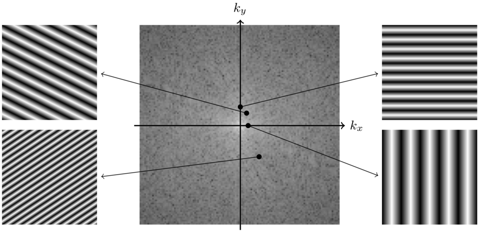 Frequency spectrum showing low/high-frequency components (Image: Felix Lugauer and Jens Wetzl, CC BY 4.0, via Wikimedia Commons)
Based on the TU BCA syllabus for Image Processing, unit 3.
Discussion
Loading…