Data Analysis and VisualizationUnit 1012 min read
OR Models & Linear Programming: Formulation, Graphs & Optimization
Unit 10 of Data Analysis and Visualization introduces Operations Research (OR) models—mathematical frameworks for decision-making—and Linear Programming (LP), a core OR technique. Learn how to formulate real-world problems as LP models, solve them graphically and algebraically, and interpret optimal solutions. Includes
TAKEAWAYS:
- OR models translate real-world problems into mathematical frameworks to find optimal decisions under constraints.
- Linear Programming solves optimization problems with linear objective functions and constraints using graphical or simplex methods.
- The graphical method visualizes feasible regions and corner points to identify optimal solutions for 2-variable problems.
- Sensitivity analysis examines how changes in constraints or objectives affect the solution.
- LP applications include production planning (e.g., Daraz’s warehouse allocation), diet optimization (e.g., Ncell’s employee meal plans), and network routing (e.g., Pathao’s delivery paths).
- Shadow prices reveal the marginal value of relaxing constraints, critical for cost-benefit analysis in projects.
1. What is Operations Research (OR)?
Operations Research (OR) is the application of mathematical models, statistics, and algorithms to solve complex decision-making problems in business, engineering, and government. It bridges the gap between real-world problems and quantitative solutions by:
- Formulating problems mathematically (e.g., constraints, objectives).
- Analyzing trade-offs (e.g., cost vs. time, profit vs. risk).
- Optimizing decisions (e.g., maximizing profit, minimizing cost).
Key OR Models (Beyond LP)
While this unit focuses on Linear Programming, OR includes:
| Model | Purpose | Example Applications |
|---|---|---|
| Queuing Theory | Optimize wait times in systems | Bank customer service, NTC call centers |
| Inventory Models | Balance stock levels and costs | Daraz’s warehouse management |
| Transportation | Minimize shipping costs | Kathmandu Valley traffic routing |
| Game Theory | Strategic decision-making | NEPSE stock market bidding |
| Simulation | Model complex systems | Pathao’s driver dispatch algorithms |
2. Linear Programming (LP): Core Concepts
LP solves problems where:
- Objective: Maximize/minimize a linear function (e.g., profit, cost).
- Constraints: Linear inequalities/equations (e.g., resource limits, demand).
- Variables: Decision variables (e.g., units produced, routes taken).
Standard LP Formulation
For a maximization problem:
Maximize  Z = c₁x₁ + c₂x₂ + ... + cₙxₙ
Subject to:
  a₁₁x₁ + a₁₂x₂ + ... + a₁ₙxₙ ≤ b₁  (Constraint 1)
  a₂₁x₁ + a₂₂x₂ + ... + a₂ₙxₙ ≤ b₂  (Constraint 2)
  ...
  x₁, x₂, ..., xₙ ≥ 0
- Z: Objective function (e.g., profit).
- xᵢ: Decision variables (e.g., product quantities).
- aᵢⱼ, bᵢ: Coefficients and resource limits.
REAL WORLD: LP in Nepal
Daraz’s Warehouse Allocation
- Problem: Distribute inventory across 3 warehouses to minimize shipping costs while meeting demand.
- LP Use: Formulate constraints for warehouse capacity, demand, and shipping costs. Solve to find the optimal allocation.
- Example:
- Variables: = units shipped from Warehouse 1, 2, 3.
- Objective: Minimize (cost per unit).
- Constraints:
- (demand).
- (Warehouse 1 capacity).
Ncell’s Network Optimization
- Problem: Place cell towers to cover maximum users with minimal towers.
- LP Use: Binary variables (1 = tower placed, 0 = not placed) and constraints for coverage areas.
Khalti’s Loan Approval
- Problem: Approve loans to maximize profit while minimizing default risk.
- LP Use: Constraints on credit scores, loan amounts, and default probabilities.
3. Solving LP Problems: Graphical Method
For problems with 2 variables, the graphical method visualizes the feasible region and finds the optimal solution at a corner point.
Step-by-Step Process
Plot Constraints:
- Convert inequalities to equations (e.g., → ).
- Shade the feasible region (area satisfying all constraints).
Identify Corner Points:
- Intersections of constraint lines (and axes).
- These are potential optimal solutions.
Evaluate Objective Function:
- Calculate at each corner point.
- For maximization, pick the highest ; for minimization, the lowest.
WORKED EXAMPLE: Daraz’s Production Plan Problem: A factory produces two products, A and B.
- Profit: A = ₹500/unit, B = ₹800/unit.
- Constraints:
- Labor: hours (max).
- Material: kg.
- Demand: , .
- Goal: Maximize profit .
Solution Steps
- Plot Constraints:
flowchart LR
  A["Labor: 2x + 3y ≤ 120"] --> B["Material: 4x + 2y ≤ 160"]
  B --> C["Demand: x ≤ 30, y ≤ 40"]
  C --> D["Feasible Region: Shaded Area"]
  D --> E["Corner Points: (0,0), (0,40), (20,20), (30,0)"]
- Graph:
- Graph:
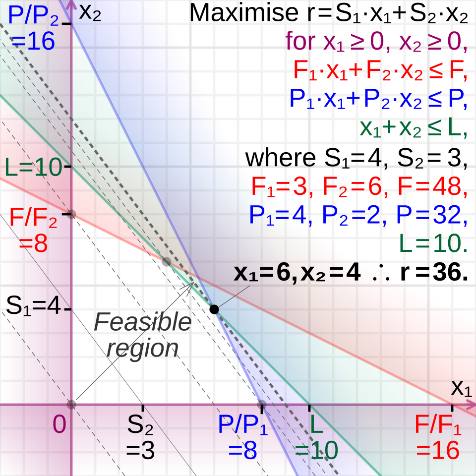 Feasible region with constraints and corner points labeled. (Image: Cmglee, CC BY-SA 4.0, via Wikimedia Commons)
```
Feasible region with constraints and corner points labeled. (Image: Cmglee, CC BY-SA 4.0, via Wikimedia Commons)
```
Find Corner Points:
- Intersection of and : Solve simultaneously: Substitute into material constraint: → , . Point: (20, 20) [Correction: Solving gives (20, 20) as the intersection].
Evaluate at Corner Points:
Point (x, y) Z = 500x + 800y (0, 0) 0 (0, 40) 32,000 (20, 20) 26,000 (30, 0) 15,000 Optimal Solution: Produce 0 units of A and 40 units of B for maximum profit of ₹32,000.
WHY THIS MATTERS:
- Daraz could use this to decide how many of Product A vs. B to stock in each warehouse.
- Ncell could apply this to optimize tower placements for coverage.
4. LP Assumptions and Limitations
Assumptions
- Linearity: Relationships between variables are linear (e.g., profit per unit is constant).
- Divisibility: Variables can take fractional values (e.g., produce 20.5 units).
- Certainty: All coefficients and constraints are known and fixed.
- Additivity: Total effect is the sum of individual effects.
Limitations
| Limitation | Real-World Impact | Example |
|---|---|---|
| Ignores uncertainty | No risk analysis (e.g., demand fluctuations) | Daraz’s stockouts during festivals |
| Linear relationships | Real-world problems often nonlinear | Diminishing returns in production |
| Divisibility constraint | May not allow integer solutions | Number of trucks must be whole |
5. Sensitivity Analysis
After solving an LP, sensitivity analysis answers:
- How much can a constraint’s RHS change before the optimal solution changes?
- How much can an objective coefficient change without altering the optimal corner point?
Key Terms
- Shadow Price: The change in the objective function value per unit increase in the RHS of a constraint.
- Example: If the shadow price for labor is ₹200/hour, increasing labor by 1 hour increases profit by ₹200.
- Range of Optimality: How much an objective coefficient can change without changing the optimal solution.
- Range of Feasibility: How much a constraint’s RHS can change without changing the shadow price.
WORKED EXAMPLE: Daraz’s Labor Constraint From the earlier example, suppose the shadow price for labor is ₹200/hour.
- Interpretation: Daraz should be willing to pay up to ₹200 extra per hour of labor to increase production capacity.
- Range of Feasibility: If labor constraint changes from 120 to 150 hours, the shadow price remains ₹200.
6. Integer and Mixed-Integer Programming
In reality, some variables must be integers (e.g., number of trucks, employees).
- Integer Programming (IP): All variables are integers.
- Mixed-Integer Programming (MIP): Some variables are integers, others continuous.
Example: NTC’s Bus Routing
- Problem: Assign buses to routes with integer constraints (can’t send 0.5 buses).
- Formulation:
- Variables: = number of buses on route .
- Constraints: must be integers.
Solving IP/MIP
- Branch and Bound: Systematic search for integer solutions.
- Cutting Planes: Adds constraints to eliminate fractional solutions.
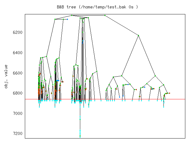 A decision tree showing how fractional solutions are split into integer branches. (Image: Xypron, GPL, via Wikimedia Commons)
7. Duality in Linear Programming
Every LP problem has a dual problem that provides insights like:
- Shadow prices (from the dual’s objective coefficients).
- Optimal value bounds.
Primal vs. Dual
| Primal (Original) | Dual |
|---|---|
| Maximize | Minimize |
| Subject to | Subject to |
Example: Dual of Daraz’s Problem
Primal (Maximize Profit):
Max Z = 500x + 800y
s.t.
  2x + 3y ≤ 120 (Labor)
  4x + 2y ≤ 160 (Material)
  x, y ≥ 0
Dual (Minimize Cost):
Min W = 120y₁ + 160y₂
s.t.
  2y₁ + 4y₂ ≥ 500 (Profit for A)
  3y₁ + 2y₂ ≥ 800 (Profit for B)
  y₁, y₂ ≥ 0
- Interpretation: The dual finds the minimum cost to achieve the given profit levels.
8. Transportation Problem (Preview of Unit 11)
A special LP where:
- Goal: Minimize transportation costs.
- Variables: = units shipped from source to destination .
- Constraints: Supply = demand.
Example: Kathmandu Traffic Routing
- Sources: 3 depots (A, B, C) with supplies 100, 150, 200 units.
- Destinations: 3 zones (X, Y, Z) with demands 120, 180, 150 units.
- Costs: per unit (e.g., A→X costs ₹5/unit).
Formulation:
Minimize Z = 5x₁₁ + 6x₁₂ + ... + 8x₃₃
s.t.
  x₁₁ + x₁₂ + x₁₃ = 100 (Depot A)
  x₂₁ + x₂₂ + x₂₃ = 150 (Depot B)
  x₃₁ + x₃₂ + x₃₃ = 200 (Depot C)
  x₁₁ + x₂₁ + x₃₁ = 120 (Zone X)
  ... (other demand constraints)
  x_{ij} ≥ 0
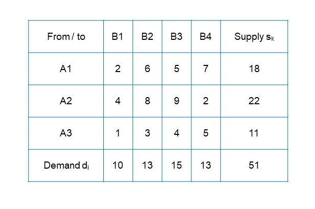 A cost matrix with supplies, demands, and routes. (Image: RVahrenkamp, CC BY-SA 4.0, via Wikimedia Commons)
Exam Tip
Formulation is 50% of the marks:
- Clearly define variables, objective, and constraints.
- Use real-world examples (e.g., Daraz, Ncell) to justify your model.
Graphical Method:
- Always label axes, shade the feasible region, and mark corner points.
- For exam questions, show all steps (even if time-consuming).
Sensitivity Analysis:
- If asked, calculate shadow prices and interpret them (e.g., "The factory should pay up to ₹200 more per hour of labor").
Duality:
- Know how to write the dual of a given primal (and vice versa).
- Understand that primal optimal = dual optimal.
Common Pitfalls:
- Non-binding constraints: Ignore them in sensitivity analysis.
- Unbounded solutions: Check if the feasible region is unbounded (e.g., no upper limit on or ).
- Infeasibility: Ensure constraints are consistent (e.g., total supply ≥ total demand in transportation problems).
PRO TIP:
- For word problems, draw a table to organize data before formulating LP.
- For graphical solutions, use grid paper to plot accurately (examiners reward precision).
RECAP VISUAL:
mindmap
  root((Linear Programming))
    Concepts
      Objective Function
      Constraints
      Feasible Region
    Methods
      Graphical Method
      Simplex Method
      Duality
    Applications
      Production Planning
      Transportation
      Resource Allocation
    Extensions
      Integer Programming
      Sensitivity Analysis
Based on the TU BCA syllabus for Data Analysis and Visualization (CACS455), unit 10.
Discussion
Loading…