Machine LearningUnit 111 min read
Introduction to ML & Data Preprocessing: Definitions, Types, Workflow & Techniques
Unit 1 of Machine Learning: Explains ML definitions, types (supervised/unsupervised/reinforcement), key workflows, and core preprocessing steps (cleaning, normalization, feature engineering) with real-world examples and step-by-step math.
TAKEAWAYS
- Machine learning is about training models from data, not hardcoding rules (e.g., spam filters in eSewa use ML to detect fraudulent transactions).
- Supervised learning uses labeled data (e.g., classifying emails as spam/not spam), while unsupervised learning finds hidden patterns (e.g., Khalti groups users by spending habits).
- Data preprocessing (cleaning, normalization, encoding) is 80% of ML success—garbage in, garbage out (e.g., Daraz’s recommendation engine relies on clean product data).
- Bias-variance tradeoff explains why overfitting (memorizing noise) or underfitting (missing trends) ruins models (e.g., a loan approval system must balance accuracy and fairness).
- Feature engineering transforms raw data into useful patterns (e.g., Pathao’s ride-demand prediction uses time-of-day encoding).
- Evaluation metrics (accuracy, precision, recall) measure model performance—confusion matrices turn raw predictions into actionable insights.
1. What is Machine Learning?
Machine learning (ML) is a subset of artificial intelligence (AI) where systems learn from data instead of following explicit instructions. Unlike traditional programming (e.g., "if temperature > 30, turn on AC"), ML models adapt to new inputs by identifying patterns.
Key Definitions
- Learning: Improving performance on a task with experience (data).
- Generalization: Model works well on unseen data (not just training data).
- Feature: A measurable property (e.g., word "offer" in spam detection).
- Label: The correct output (e.g., "spam" or "not spam").
Types of Machine Learning
flowchart TD
    A["Machine Learning"] --> B["Supervised Learning"]
    A --> C["Unsupervised Learning"]
    A --> D["Reinforcement Learning"]
    B --> B1["Classification\n(e.g., spam/not spam)"]
    B --> B2["Regression\n(e.g., house price prediction)"]
    C --> C1["Clustering\n(e.g., customer segmentation)"]
    C --> C2["Dimensionality Reduction\n(e.g., visualizing high-dimensional data)"]
    D --> D1["Agents learn via rewards\n(e.g., self-driving cars)"]
Real-world tie:
- eSewa’s fraud detection uses supervised learning (classification) to flag suspicious transactions based on labeled historical data (e.g., "high transaction amount + unusual location = fraud").
- Khalti’s user segmentation uses unsupervised learning (clustering) to group customers by spending behavior without predefined labels.
2. Why Learn Machine Learning?
ML automates tasks that are:
- Too complex for rules (e.g., recognizing faces in photos).
- Too repetitive (e.g., sorting emails).
- Too large for humans (e.g., analyzing NEPSE stock trends).
Example: Daraz’s Recommendations Daraz uses ML to suggest products based on:
- Collaborative filtering (users who bought X also bought Y).
- Content-based filtering (items similar to what you liked).
- Deep learning (image recognition for product tags).
3. Machine Learning Workflow
A typical ML project follows this pipeline:
flowchart LR
    A["Problem Definition"] --> B["Data Collection"]
    B --> C["Data Preprocessing"]
    C --> D["Feature Engineering"]
    D --> E["Model Selection"]
    E --> F["Training"]
    F --> G["Evaluation"]
    G --> H["Deployment"]
    H --> I["Monitoring"]
Step 1: Problem Definition
- Classification: Predict categories (e.g., "spam" or "not spam").
- Regression: Predict continuous values (e.g., house price).
- Clustering: Group similar items (e.g., customer segments).
- Reinforcement Learning: Learn via rewards (e.g., robotics).
Worked Example: Spam Filter (Past Exam Question) Given:
| Class | P(offer) | P(win) | Prior Probability |
|---|---|---|---|
| Spam | 0.8 | 0.6 | 0.4 |
| Not Spam | 0.1 | 0.05 | 0.6 |
Question: Classify an email with words "offer" and "win."
Solution (Naive Bayes):
- Calculate joint probability for each class:
- P(Spam|offer,win) = P(offer|Spam) × P(win|Spam) × P(Spam) = 0.8 × 0.6 × 0.4 = 0.192
- P(Not Spam|offer,win) = 0.1 × 0.05 × 0.6 = 0.003
- Compare probabilities: Spam (0.192 > 0.003).
Answer: The email is classified as Spam.
4. Data Preprocessing: Cleaning the Data
Real-world data is dirty. Preprocessing fixes issues like:
- Missing values (e.g., "N/A" in employee ages).
- Outliers (e.g., a salary of ₹100 million in a dataset of ₹10k salaries).
- Inconsistent formats (e.g., "USA" vs. "US").
Key Techniques
| Technique | Description | Example |
|---|---|---|
| Handling Missing Data | Impute (fill) or remove missing values. | Replace "?" with median age. |
| Normalization | Scale features to [0,1] or [-1,1] (e.g., Min-Max: (x - min)/(max - min)). |
Resize pixel values in an image. |
| Encoding | Convert categorical data to numbers (e.g., "Male" → 1, "Female" → 0). | One-Hot Encoding for "Red/Green/Blue". |
| Feature Engineering | Create new features from raw data (e.g., "age_group" from age). | Bin ages into "Young (≤30), Middle (31-50), Senior (>50)". |
Worked Example: Employee Ages (Past Exam) Given ages: [22, 25, 29, 30, 31, 33, 35, 36, 40, 45]
a. Descriptive Statistics
- Minimum: 22
- Q1 (25th percentile): 29
- Median (50th percentile): 32.5
- Q3 (75th percentile): 36
- Maximum: 45
b. Box Plot
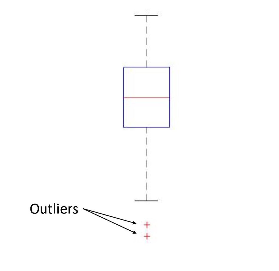
(Visual: A box from Q1 to Q3, median line inside, whiskers to min/max, no outliers.)
5. Feature Engineering
Raw data is often useless. Feature engineering transforms it into useful patterns.
Techniques
- Binning: Convert continuous data into categories.
- Example: Age → "Young", "Middle-aged", "Senior".
- Polynomial Features: Add interaction terms.
- Example: For price (
P) and size (S), createP²,P×S.
- Example: For price (
- Text Processing: Convert words to numbers (e.g., TF-IDF for spam detection).
- Time-Based Features: Extract day/hour from timestamps (e.g., for Pathao’s demand prediction).
Example: Pathao’s Ride Demand Prediction
- Raw Data: Timestamp, pickup location, weather.
- Engineered Features:
- Hour of day (0-23).
- Day of week (Monday=1, Sunday=7).
- Distance from nearest station.
6. Bias-Variance Tradeoff
A model’s error comes from two sources:
- Bias: Error from oversimplification (underfitting).
- Variance: Error from overfitting to noise.
flowchart TD
    A["High Bias
(Underfitting)"] -->|Model too simple| B["High Variance
(Overfitting)"]
    C["Complex Model"] --> B
    D["Simple Model"] --> A
    A -->|"Error from oversimplification"| E["High Bias"]
    B -->|"Error from overfitting"| F["High Variance"]
    E -->|"Model too simple"| A
    F -->|"Model too complex"| C
Example: Loan Approval System
- High Bias: Always rejects loans (too simple rule).
- High Variance: Approves loans based on tiny fluctuations (e.g., "approved if applicant’s name starts with 'A'").
- Balanced Model: Uses credit score + income + employment history.
7. Model Evaluation Metrics
| Metric | Formula | When to Use |
|---|---|---|
| Accuracy | TP + TN / Total | Balanced classes. |
| Precision | TP / (TP + FP) | Avoid false positives (e.g., spam). |
| Recall | TP / (TP + FN) | Catch all positives (e.g., fraud). |
| F1-Score | 2 × (Precision × Recall) / (P+R) | Balance precision/recall. |
Confusion Matrix Example
(Visual: 2x2 table with TP, FP, FN, TN labeled.)
Worked Example: K-NN (Past Exam) Given dataset:
| Day | Outlook | Temperature | Humidity | Wind | Decision |
|---|---|---|---|---|---|
| 1 | Sunny | Hot | High | Weak | Yes |
| 2 | Sunny | Hot | High | Strong | No |
New Example: Sija = {Machine Learning=60, GIS=80} (Assume features are "score in ML" and "score in GIS".) Steps:
- Calculate distance to each point (Euclidean distance).
- Find 3 nearest neighbors (k=3).
- Majority vote: If 2+ neighbors say "Yes," predict "Yes."
8. Dimensionality Reduction
High-dimensional data is hard to visualize/process. Techniques like PCA reduce dimensions while preserving variance.
Example: NEPSE Stock Trends
- Original Data: 50 features (e.g., price, volume, moving averages).
- Reduced Data: 2-3 features (e.g., "trend strength" + "volatility").
- Visualization:
In the Real World
eSewa’s Fraud Detection
- Idea: Supervised learning (classification) with features like transaction amount, location, and user history.
- How: Trained on labeled data (fraudulent/legitimate) to flag suspicious transactions in real time.
Khalti’s User Segmentation
- Idea: Unsupervised learning (clustering) to group customers by spending behavior.
- How: Uses K-means to identify high-value vs. low-value users for targeted promotions.
Pathao’s Ride Demand Prediction
- Idea: Time-series forecasting + feature engineering.
- How: Models hour-of-day, weather, and location data to predict demand and optimize driver dispatch.
Exam Tips
For definitions:
- Always include input/output (e.g., "ML takes data → learns patterns → makes predictions").
- Compare supervised vs. unsupervised with examples (e.g., "eSewa uses supervised; Khalti uses unsupervised").
For preprocessing:
- Show math for normalization (e.g.,
(x - min)/(max - min)). - Mention why each step is needed (e.g., "Normalization helps gradient descent converge faster").
- Show math for normalization (e.g.,
For bias-variance tradeoff:
- Draw a graph of error vs. model complexity (U-shaped curve).
- Relate to real examples (e.g., "A loan model that’s too simple misses good applicants (high bias).")
For evaluation metrics:
- Always define TP/FP/FN/TN before the confusion matrix.
- For imbalanced data (e.g., spam vs. not spam), emphasize precision/recall over accuracy.
For worked examples:
- Show step-by-step calculations (e.g., Naive Bayes probabilities).
- Assume small numbers (e.g., 2-3 data points) to keep it simple.
Final Note: ML is about turning data into decisions. Master the workflow, preprocessing, and evaluation—these are 90% of the exam!
Based on the TU BCA syllabus for Machine Learning (CACS486), unit 1.
Discussion
Loading…