Multimedia SystemUnit 510 min read
Data Compression Techniques: Lossless vs. Lossy, Algorithms & Applications
Unit 5 of Multimedia System explores how data compression reduces file sizes while preserving or sacrificing quality, covering lossless (RLE, Huffman, LZW) and lossy (DCT, quantization) methods, their mathematical foundations, and real-world trade-offs in video, audio, and storage systems.
TAKEAWAYS:
- Lossless compression (e.g., Huffman coding) recovers original data perfectly but achieves lower ratios (e.g., 2:1) than lossy methods.
- Lossy compression (e.g., JPEG’s DCT) sacrifices quality for higher ratios (e.g., 10:1–100:1) by exploiting human perception limits.
- Run-Length Encoding (RLE) works best for data with repeated symbols (e.g., fax scans), while arithmetic coding achieves near-entropy limits.
- Video compression (MPEG) combines spatial (DCT) and temporal (motion estimation) techniques to reduce redundancy.
- Compression algorithms trade computational cost (e.g., Huffman table building) against speed (e.g., LZW’s fixed dictionary).
- Real-world systems (e.g., WhatsApp’s image compression, Ncell’s video streaming) use hybrid approaches to balance quality and bandwidth.
1. Why Compress Data? The Core Problem
Data compression reduces storage/transmission requirements by removing redundancy (repeated patterns) or irrelevant information (perceptually insignificant details). Without compression:
- A 4K video (8 GB/hour) would exhaust mobile data in minutes.
- WhatsApp would need servers 10× larger to store chats.
- Ncell’s 5G network would collapse under raw video calls.
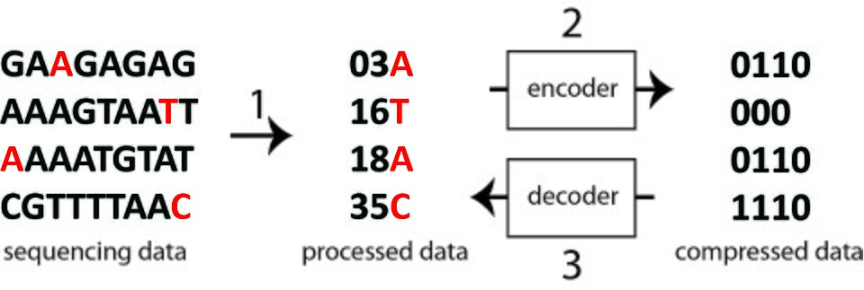 Shows input data → redundancy removal → compressed output → decompression → reconstructed data. (Image: Medgener123, CC BY-SA 3.0, via Wikimedia Commons)
2. Lossless Compression: Perfect Reconstruction
Definition: Algorithms that reconstruct the exact original data after decompression. Used for text, spreadsheets, and medical images where no data loss is tolerable.
A. Run-Length Encoding (RLE)
How it works:
- Replaces consecutive identical symbols with a count + symbol pair.
- Example:
"aaaaabbbbcccdde"→(5,a)(4,b)(3,c)(2,d)(1,e).
Worked Example: Daraz Order Queue
Suppose Daraz’s backend logs orders as:
"P1,P1,P2,P3,P1,P1,P1,P4,P5,P5,P5,P5,P6"
RLE compresses this to:
(3,P1)(1,P2)(1,P3)(3,P1)(1,P4)(4,P5)(1,P6)
Compression ratio: Original (12 bytes) → Compressed (12 bytes, but often smaller for longer runs).
Limitations:
- Fails on random data (e.g.,
"abcabcabc"→ no compression). - Best for binary images (e.g., fax scans) or simple patterns.
B. Huffman Coding
How it works:
- Frequency analysis: Count symbol occurrences (e.g., in
"mississippi",'i'appears 4×,'s'4×,'p'2×). - Build a binary tree: Assign shorter codes to frequent symbols.
- Example tree:
i(4), s(4) / \ p(2) m(1) - Codes:
'i'=00,'s'=01,'p'=10,'m'=110.
- Example tree:
- Encode: Replace symbols with their codes (
"mississippi"→110 1100 01 01 00 01 01 00 01 00).
Advantages:
- Optimal for symbol frequencies: Achieves near-entropy limits (theoretical max compression).
- Used in PKZIP, PNG, TIFF.
Disadvantage:
- Requires a decoder-side frequency table (metadata overhead).
Worked Example: NTC Electricity Bill Data
Suppose NTC stores monthly usage as:
"120,120,120,121,121,122,122,122,123,123,123,123"
Huffman coding (after frequency analysis) might assign:
'120'=0,'121'=10,'122'=110,'123'=111. Compressed:0,0,0,10,10,110,110,110,111,111,111,111.
C. Lempel-Ziv-Welch (LZW)
How it works:
- Builds a dynamic dictionary of repeated phrases.
- Example: Compress
"ABABABABAB":- Start with dictionary
{A:0, B:1}. - Encounter
"AB"(not in dict) → assign2, add to dict. - Next
"AB"→ output2, repeat. Output:0,1,2,2,2,2(original: 10 bytes → compressed: 6 bytes).
- Start with dictionary
Applications:
- GIF, TIFF, ZIP formats.
- WhatsApp images: Uses LZW-like methods to reduce size before JPEG compression.
Limitations:
- Slower than Huffman for static data.
- Dictionary grows with input size.
3. Lossy Compression: Sacrificing Quality for Gain
Definition: Permanently discards perceptually irrelevant data. Used for audio, video, and photos where minor quality loss is acceptable.
flowchart TD
    A["Original Frame"] --> B["Divide into 8x8 Blocks"]
    B --> C["Apply DCT"]
    C --> D["Quantize High Frequencies"]
    D --> E["Huffman Encode"]
    E --> F["Compressed JPEG"]
JPEG compression pipeline (DCT + quantization + entropy coding).A. Discrete Cosine Transform (DCT) in JPEG
How it works:
- Divide image into 8×8 blocks.
- Apply DCT: Converts spatial data (pixels) to frequency components (like a Fourier transform but for 2D).
- Quantization: Divide high-frequency coefficients (edges/details) by large numbers → loss of precision.
- Entropy coding: Huffman/RLE on quantized coefficients.
Why it works:
- Human eyes are less sensitive to high frequencies (blurry edges).
- Example: A
512×512JPEG at 90% quality discards ~70% of DCT coefficients.
B. Motion Estimation in MPEG
How it works:
- Temporal redundancy: Consecutive video frames are nearly identical.
- Keyframes (I-frames): Full images stored every few seconds.
- Predicted frames (P-frames): Store only motion vectors (e.g., "pixel at (x,y) moved to (x+2,y-1)").
- Bidirectional frames (B-frames): Use past/future frames for interpolation.
Example: Pathao Driver’s Video Call
- Original: 30 fps × 1080p = 10 Mbps.
- Compressed: I-frame every 0.5s + P-frames = ~1 Mbps (90% reduction).
4. Lossless vs. Lossy: Comparison Table
| Feature | Lossless | Lossy |
|---|---|---|
| Reconstruction | Exact original data | Approximate (quality loss) |
| Compression Ratio | 2:1 to 5:1 | 10:1 to 100:1 |
| Use Cases | Text, code, medical images | Audio, video, photos |
| Algorithms | Huffman, LZW, RLE | DCT (JPEG), MP3, MPEG |
| Computational Cost | Low (except LZW) | High (DCT, motion estimation) |
| Real-World Example | WhatsApp chat backups | YouTube videos, Ncell 4G streaming |
5. Hybrid Compression: The Best of Both Worlds
Many systems combine lossless and lossy:
- Lossy first: Reduce data size (e.g., JPEG for photos).
- Lossless second: Compress metadata (e.g., Huffman on DCT coefficients).
Example: Google Photos
- Step 1: Apply lossy JPEG compression (20:1 ratio).
- Step 2: Apply lossless WebP format (additional 10% reduction).
- Result: A 2 MB photo becomes ~100 KB.
In the Real World
WhatsApp Image Compression
- How: Uses lossy JPEG + lossless LZW to reduce size before upload.
- Impact: Saves ~60% bandwidth vs. uncompressed photos.
- Example: A 3 MB iPhone photo → ~1.2 MB after WhatsApp compression.
Ncell’s 4G Video Streaming
- How: MPEG-4 (H.264) with adaptive bitrate (switches between lossy levels based on network).
- Impact: Delivers 720p smoothly on 3G by dropping high-frequency details.
- Example: A 10 MB/s raw video → ~1.5 MB/s after compression.
Daraz’s Order Database
- How: Lossless RLE + Huffman on repeated order IDs (e.g.,
"P1,P1,P1,P2"→(3,P1)(1,P2)). - Impact: Reduces database size by ~40% without losing transaction records.
- How: Lossless RLE + Huffman on repeated order IDs (e.g.,
Exam Tip
For RLE/Huffman questions:
- Always show the step-by-step encoding/decoding.
- Calculate compression ratio as:
Ratio = (Uncompressed Size) / (Compressed Size). - Example:
"aaaaabbbb"(8 bytes) →(5,a)(4,b)(4 bytes) → Ratio = 2:1.
For lossy vs. lossless comparisons:
- JPEG (lossy) uses DCT + quantization → higher ratio but quality loss.
- PNG (lossless) uses Huffman + LZW → no quality loss but lower ratio.
- Mention perceptual models (e.g., "human eye ignores high frequencies").
For video compression:
- MPEG combines:
- Spatial compression (DCT like JPEG).
- Temporal compression (motion estimation).
- Keyframes (I-frames) are stored fully; P/B-frames store differences.
- MPEG combines:
Common pitfalls:
- Don’t confuse RLE with Huffman: RLE is for runs; Huffman is for frequencies.
- Lossy ≠ "bad": It’s essential for video/audio where bandwidth matters more than perfection.
- Always justify: If asked why lossy is preferred for 4K video, say:
"4K video has massive spatial/temporal redundancy. Lossy methods (e.g., H.265) exploit perceptual limits (e.g., masking high frequencies) to reduce bitrate from ~100 Mbps to ~5–10 Mbps without noticeable quality loss."
flowchart TD
    A["Input Data"] --> B["Redundancy Analysis"]
    B --> C["Choose Method"]
    C --> D["Lossless Path"]
    C --> E["Lossy Path"]
    D --> F["RLE/Huffman/LZW"]
    E --> G["DCT/Quantization"]
    F --> H["Exact Reconstruction"]
    G --> I["Perceptual Approximation"]
    H --> J["Output: Original Data"]
    I --> K["Output: Compressed Data"]
    J --> L["Applications: Text, Code"]
    K --> M["Applications: Video, Audio"]
In the real world
- WhatsApp Image Compression: Uses lossy JPEG + lossless LZW to reduce a 3 MB iPhone photo to ~1.2 MB (60% bandwidth saved) before upload. The lossy step discards perceptually irrelevant details, while LZW compresses metadata losslessly.
- Ncell 4G Video Streaming: Employs MPEG’s motion estimation (P/B-frames) to cut a 10 Mbps 1080p call to ~1 Mbps, enabling smooth streaming on limited bandwidth. Keyframes (I-frames) are stored every 0.5 seconds.
- Daraz Order Processing: Uses RLE for repeated order IDs (e.g.,
P1,P1,P1→(3,P1)) in backend logs, reducing storage needs for high-volume transactions.
Based on the TU BCA syllabus for Multimedia System (CACS457), unit 5.
Discussion
Loading…