Operational ResearchUnit 714 min read
Queuing Theory: Models, Assumptions & Real-World Applications
Unit 7 of Operational Research explores queuing theory—how to model and optimize waiting lines using mathematical techniques, including single-channel systems, arrival patterns, service rates, and cost-benefit analysis. This note covers definitions, key models, assumptions, and practical applications in Nepalese and gl
TAKEAWAYS:
- Queuing theory analyzes waiting lines (queues) to minimize costs and improve efficiency using arrival rates (λ), service rates (μ), and queue discipline.
- The M/M/1 model (Markovian arrivals and service) is the simplest single-channel queue, where customers wait in a line for one server (e.g., a bank teller).
- Key metrics like average queue length (Lq), waiting time (Wq), and system time (Ws) are derived from Little’s Law: .
- Assumptions (e.g., Poisson arrivals, exponential service times) simplify real-world problems but must be checked for validity.
- Applications range from call centers (Ncell) to e-commerce order processing (Daraz) and traffic management (Kathmandu’s ring road).
- Exam focus: Compare models, solve for metrics, and justify assumptions in real-world scenarios (e.g., a hospital’s emergency ward).
1. Introduction to Queuing Theory
Queuing theory is a branch of Operational Research (OR) that studies waiting lines (queues) to optimize service systems. It helps businesses and governments reduce costs, improve customer satisfaction, and allocate resources efficiently.
Why Study Queuing Theory?
- Real-world impact: Delays cost money (e.g., a customer waiting at a bank loses productivity).
- Decision-making: Helps design systems like call centers, hospitals, and traffic signals.
- Mathematical foundation: Uses probability, statistics, and stochastic processes.
Key Terms
| Term | Definition |
|---|---|
| Arrival rate (λ) | Average number of customers arriving per unit time (e.g., 10 customers/hour). |
| Service rate (μ) | Average number of customers served per unit time (e.g., 8 customers/hour). |
| Queue discipline | Rule for selecting the next customer (e.g., FIFO: First-In-First-Out). |
| System capacity | Maximum number of customers the system can handle simultaneously. |
| Steady state | When arrival and service rates balance over time (queue length stabilizes). |
2. Components of a Queuing System
Every queuing system has three essential components:
- Input source: Where customers arrive (e.g., people entering a bank).
- Service facility: Where customers are served (e.g., a teller’s counter).
- Queue discipline: Rules governing the order of service (e.g., FCFS, LIFO, priority).
Visual: Queuing System Structure
flowchart LR
    A["Input Source\n(e.g., Customers)"] -->|"Arrive at rate λ"| B["Queue\n(Waiting Line)"]
    B -->|"Join queue"| C["Service Facility\n(e.g., Server/Teller)"]
    C -->|"Serve at rate μ"| D["Output\n(Served Customers)"]
    D --> A
3. Types of Queuing Models
Queuing models are classified based on:
- Arrival pattern (e.g., random, deterministic).
- Service mechanism (e.g., single-server, multi-server).
- Queue discipline (e.g., FIFO, priority).
- System capacity (e.g., finite or infinite).
Kendall’s Notation
Models are often described using Kendall’s notation: A/B/c/K/N/M
- A: Arrival process (e.g., M = Markovian/Poisson, D = Deterministic).
- B: Service time distribution (e.g., M = Markovian/exponential, G = General).
- c: Number of servers.
- K: Queue capacity (maximum number in the system).
- N: Population size (if finite).
- M: Service discipline (e.g., FCFS, LCFS).
Example: An M/M/1 model means:
- Arrivals: Poisson process (random).
- Service times: Exponentially distributed (random).
- Single server.
4. Single-Channel Queuing Model (M/M/1)
The M/M/1 model is the simplest queuing system:
- One server (e.g., a single bank teller).
- Poisson arrivals (λ customers/hour).
- Exponential service times (μ customers/hour).
- Infinite queue capacity (customers can wait indefinitely).
Assumptions of M/M/1 Model
- Arrivals follow a Poisson process (probability of arrival is independent of past events).
- Service times are exponentially distributed (memoryless property).
- The system is stable (λ < μ, otherwise the queue grows infinitely).
- First-Come-First-Served (FCFS) discipline.
- Infinite queue capacity (no maximum limit on waiting customers).
Key Metrics for M/M/1
For an M/M/1 system in steady state (λ < μ), the following metrics are derived:
Probability of an empty system (P₀):
Average number of customers in the queue (Lq):
Average number of customers in the system (L):
Average waiting time in the queue (Wq):
Average time in the system (Ws):
Worked Example 1: Bank Teller Queue
Scenario: A bank has one teller serving customers. Customers arrive at a rate of λ = 12 per hour, and the teller serves customers at a rate of μ = 15 per hour. Assume Poisson arrivals and exponential service times.
Questions:
- What is the probability that the bank is empty?
- What is the average number of customers waiting in the queue?
- What is the average waiting time for a customer?
Solution:
Probability of an empty system (P₀):
Average queue length (Lq):
Average waiting time (Wq):
Visual: Queue Length Distribution This graph shows the probability of having n customers in the system. The probability decreases as n increases.
5. Real-World Applications of Queuing Theory
Queuing theory is used in Nepal and globally to optimize systems where waiting occurs. Here’s how:
Example 1: Ncell Customer Service Center (M/M/c Model)
- Problem: Ncell receives λ = 200 calls/hour, but their 3 customer service agents handle μ = 80 calls/hour each.
- Issue: Long wait times frustrate customers.
- Solution: Queuing theory helps determine:
- How many agents are needed to keep wait times under 2 minutes.
- Whether adding a 4th agent reduces costs more than it increases wages.
- Key Metric: Use Erlang C formula (for multi-server queues) to calculate: Here, . If minutes, more agents are needed.
Example 2: Daraz Order Fulfillment (M/G/1 Model)
- Problem: Daraz’s warehouse processes λ = 500 orders/day, but order processing times vary (some take 5 minutes, others 30 minutes).
- Issue: Customers complain about delayed deliveries.
- Solution: Queuing theory helps:
- Model variable service times (G) to predict delays.
- Optimize warehouse staffing during peak hours (e.g., Dashain sales).
- Key Metric: Use Pollaczek-Khinchine formula for M/G/1: If minutes and variance is high, Daraz may prioritize faster orders or hire temporary staff.
Example 3: Kathmandu Traffic Management (M/M/∞ Model)
- Problem: Traffic jams at Kathmandu’s Ring Road cause λ = 1000 vehicles/hour to enter a single lane, but the lane can only handle μ = 600 vehicles/hour.
- Issue: Long queues and accidents.
- Solution: Queuing theory helps:
- Model traffic flow as M/M/1 to predict congestion.
- Design smart traffic lights to dynamically adjust green/red times.
- Key Metric: Calculate probability of delay using: Solution: Add more lanes or restrict entry during peak hours.
6. Multi-Channel Queuing Models
When a system has multiple servers, the model becomes M/M/c (e.g., a bank with 3 tellers).
Key Differences: M/M/1 vs. M/M/c
| Feature | M/M/1 (Single Server) | M/M/c (Multi-Server) |
|---|---|---|
| Servers | 1 | c (e.g., 2, 3, or more) |
| Queue Length | More complex (Erlang C formula) | |
| Utilization (ρ) | ||
| Example | Single ATM | Bank with 3 tellers |
Worked Example 2: Hospital Emergency Ward (M/M/c)
Scenario: A hospital’s emergency ward has:
- λ = 20 patients/hour.
- 3 doctors, each serving at μ = 8 patients/hour.
- FCFS discipline.
Questions:
- What is the probability that all doctors are busy?
- What is the average number of patients waiting?
Solution:
Utilization per doctor (ρ): The probability that all doctors are busy is calculated using the Erlang C formula, but for simplicity, we can approximate using: (Full calculation requires solving for , but this gives an idea.)
Average queue length (Lq): Using the Erlang C formula: (Numerical solution required; typically solved using software or tables.)
7. Economic Considerations in Queuing Systems
Queuing theory isn’t just about math—it’s about cost vs. service level. Businesses must balance:
- Cost of waiting (e.g., customer dissatisfaction, lost sales).
- Cost of service (e.g., hiring more staff, buying equipment).
Cost Components
| Cost Type | Example |
|---|---|
| Waiting Cost (Cw) | Lost productivity, frustration (e.g., a customer waiting at a bank). |
| Service Cost (Cs) | Salaries, equipment, space (e.g., hiring a 2nd teller). |
| Total Cost (TC) |
Optimal Number of Servers
Businesses use queuing theory to find the cost-minimizing number of servers. For example:
- A call center may calculate that adding a 4th agent reduces wait times from 5 minutes to 2 minutes, saving Rs. 50,000/day in lost sales, even if it costs Rs. 30,000/day in wages.
8. Limitations of Queuing Models
While powerful, queuing models have limitations:
- Assumptions may not hold:
- Real arrivals aren’t always Poisson (e.g., rush hour traffic spikes).
- Service times may not be exponential (e.g., some orders take much longer than others).
- Complexity increases with realism:
- Adding priority queues, balking (customers leaving if the queue is too long), or reneging (customers leaving while waiting) makes models harder to solve.
- Human behavior is unpredictable:
- Customers may change their minds or complain, affecting the system.
9. Advanced Topics (Exam Relevance)
While the syllabus focuses on basic models, exams may test:
- Priority Queues: Customers with higher priority get served first (e.g., VIPs at a hospital).
- Bulk Service: A server handles multiple customers at once (e.g., a bus picking up passengers).
- Finite Population Models: Limited number of customers (e.g., machines in a factory needing repair).
Exam Tip
- Understand the assumptions: Always state whether arrivals are Poisson, service times exponential, etc.
- Know the formulas: Memorize Little’s Law, M/M/1 metrics, and Erlang C for multi-server systems.
- Relate to real-world examples:
- Ncell: Use M/M/c to optimize call center staffing.
- Daraz: Use M/G/1 for variable order processing times.
- Banks: Use M/M/1 for single-teller queues.
- Draw diagrams: Sketch the queuing system (input → queue → server → output) in exams.
- Calculate cost trade-offs: If asked about "optimal servers," show both waiting cost and service cost.
Summary Table: Queuing Models
| Model | Description | Key Formulae | Example |
|---|---|---|---|
| M/M/1 | Single server, Poisson arrivals | Single bank teller | |
| M/M/c | Multiple servers, Poisson arrivals | Erlang C formula | Call center with 5 agents |
| M/G/1 | Single server, general service times | Pollaczek-Khinchine formula | Daraz order processing |
| M/M/∞ | Infinite servers (no queue) | Traffic flow on a highway |
Practice Questions (Exam Style)
A hospital has one doctor serving patients at a rate of μ = 10 patients/hour. Patients arrive at λ = 8 patients/hour. Calculate:
- Probability the doctor is idle.
- Average number of patients in the queue.
- Average waiting time.
A fast-food restaurant has 2 counters. Customers arrive at λ = 15/hour, and each counter serves at μ = 10/hour. What is the average time a customer spends in the system?
Discuss how queuing theory can improve efficiency at:
- Nepal’s NTC bus stands.
- Khalti’s customer support.
- Pathao’s driver dispatch system.
Final Answer Structure for Exams
When answering questions on queuing theory:
- Define the model (e.g., "This is an M/M/1 queuing system...").
- State assumptions (Poisson arrivals, exponential service, etc.).
- Calculate key metrics (Lq, Wq, L, Ws).
- Interpret results (e.g., "The average wait time is 5 minutes, which may require adding a second server").
- Relate to real-world (e.g., "This applies to Ncell’s call center...").
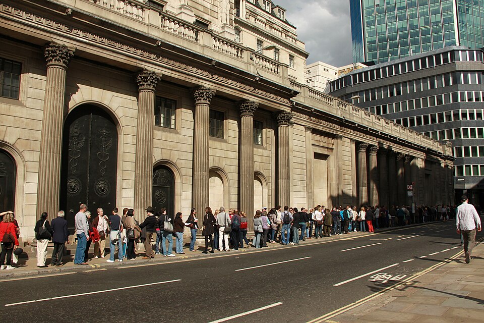 A single teller serving customers in a bank queue (M/M/1 model) (Image: Cristian Bortes from Cluj-Napoca, Romania, CC BY 2.0, via Wikimedia Commons)
 Multiple agents handling calls (M/M/c model) (Image: FiveOne51, CC BY-SA 3.0, via Wikimedia Commons)
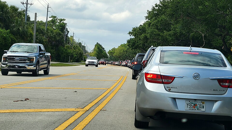 Vehicles waiting at a signal (M/M/1 with finite capacity) (Image: Kiran891, CC BY-SA 4.0, via Wikimedia Commons)
Based on the TU BCA syllabus for Operational Research (CAOR451), unit 7.
Discussion
Loading…