Transportation Problem – Formulation, Methods, and Applications

Introduction

The transportation problem is one of the most studied combinatorial optimization problems. It models the cost‑minimizing shipment of goods from a set of suppliers to a set of consumers while satisfying supply and demand constraints. Its structure is highly regular, which allows for specialized algorithms that are faster than general linear programming solvers.

Mathematical Formulation

Let there be $m$ supply nodes $S_i$ with supplies $a_i$ and $n$ demand nodes $D_j$ with demands $b_j$. The cost of shipping one unit from $S_i$ to $D_j$ is $c_{ij}$.
The decision variables are $x_{ij}$ (units shipped from $S_i$ to $D_j$).

$$\begin{array}{rl}\text{Minimize }& Z=\sum _{i=1}^m\sum _{j=1}^n{c}_{ij}{x}_{ij}\\ \text{subject to }& \sum _{j=1}^n{x}_{ij}=a_i(i=1,\dots ,m)\text{(supply)}\\ & \sum _{i=1}^m{x}_{ij}=b_j(j=1,\dots ,n)\text{(demand)}\\ & x_{ij}\ge 0\forall i,j\end{array}$$

The problem is feasible if $\sum a_i=\sum b_j$. If not, a dummy source or sink is added.

Figure – Cost Matrix

Feasible Solution Generation

Several systematic methods exist to generate an initial basic feasible solution (IBFS).

Figure – Northwest Corner Tableau

Optimality Test – MODI (Modified Distribution) Method

After obtaining an IBFS, the MODI method checks optimality by computing dual variables $u_i$ (for rows) and $v_j$ (for columns) such that for every basic cell $c_{ij}$:

$$u_i+v_j=c_{ij}$$

For non‑basic cells, compute the reduced cost $r_{ij}=c_{ij}-(u_i+v_j)$.
If all $r_{ij}\ge 0$, the solution is optimal. Otherwise, the most negative $r_{ij}$ indicates a loop to improve the solution.

Figure – Dual Variables and Reduced Costs

Worked Example – Using MODI

Problem
Supply: $S_1=30$, $S_2=40$, $S_3=20$.
Demand: $A=25$, $B=35$, $C=20$.
Cost matrix (same as above but with 3 columns):

Step 1 – IBFS (Northwest Corner)

Step 2 – Dual Variables
Set $u_1=0$.
From $S_{1}A$: $u_1+v_A=12\Rightarrow v_A=12$.
From $S_{1}B$: $u_1+v_B=14\Rightarrow v_B=14$.
From $S_{2}B$: $u_2+v_B=42\Rightarrow u_2=28$.
From $S_{2}C$: $u_2+v_C=15\Rightarrow v_C=-13$.
From $S_{3}C$: $u_3+v_C=9\Rightarrow u_3=22$.

Step 3 – Reduced Costs

The most negative reduced cost is $-6$ at $S_{3}B$.
Step 4 – Form Loop
Loop: $S_{3}B\to S_{2}B\to S_{2}C\to S_{3}C\to S_{3}B$.
Minimum allocation on loop = 10 (at $S_{2}C$).
Adjust: add 10 to $S_{3}B$, subtract 10 from $S_{2}C$.

New allocations:
$S_{3}B=10$, $S_{2}C=0$.

Step 5 – Recompute Duals
Re‑solve for duals with updated basic cells.
Resulting reduced costs are all non‑negative → optimal.

Optimal Solution

Total Cost
$Z=25(12)+5(14)+30(42)+10(30)+10(9)=300+70+1260+300+90=2020$.

Figure – Final Allocation Matrix

Dual Interpretation

The dual of the transportation problem is:

$$\begin{array}{rl}\text{Maximize }& \sum _{i=1}^m{a}_i{u}_i+\sum _{j=1}^n{b}_j{v}_j\\ \text{subject to }& u_i+v_j\le c_{ij}\forall i,j\end{array}$$

The optimal dual variables $u_i,v_j$ represent the shadow price of increasing supply at $S_i$ or demand at $D_j$. In logistics, this indicates how much the total cost would change if an extra unit were supplied or demanded.

Comparison of Solution Methods

Real‑World Applications

In the real world

1. eSewa Cash Distribution – eSewa maintains a network of ATMs across Nepal. The company uses a transportation model to decide how many cash bundles to send from central warehouses to each ATM, minimizing transport cost while meeting ATM cash demand.
2. Daraz Warehouse‑to‑Customer Routing – Daraz’s fulfillment centers supply millions of orders daily. A transportation problem determines the optimal shipment plan from multiple warehouses to city‑wide delivery hubs, reducing shipping cost and delivery time.
3. Ncell Bandwidth Allocation – Ncell allocates bandwidth from core data centers to regional base stations. The problem is analogous to transporting data packets, where the cost is latency and the supply/demand are bandwidth capacities and user demands.

These examples illustrate how the abstract transportation model directly informs operational decisions in finance, e‑commerce, and telecommunications.

Advantages & Disadvantages

Exam Tip

• Identify the type of problem: Confirm that the problem is a transportation problem (balanced supply/demand, linear costs).
• Choose the right method: For small problems, use MODI or Stepping‑stone; for larger problems, start with Vogel’s approximation to get a good IBFS.
• Check optimality: Always compute reduced costs; if any are negative, the solution is not optimal.
• Report results clearly: Provide the final allocation matrix, total cost, and dual variables if asked.
• Practice with past questions: Solve at least two full problems from the syllabus, including the example with the cost matrix above, to become comfortable with the steps.

---

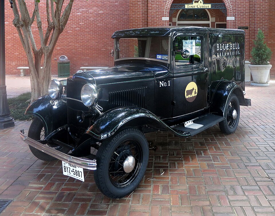Truck used in transportation problem (Image: Jim Evans, CC BY-SA 4.0, via Wikimedia Commons) 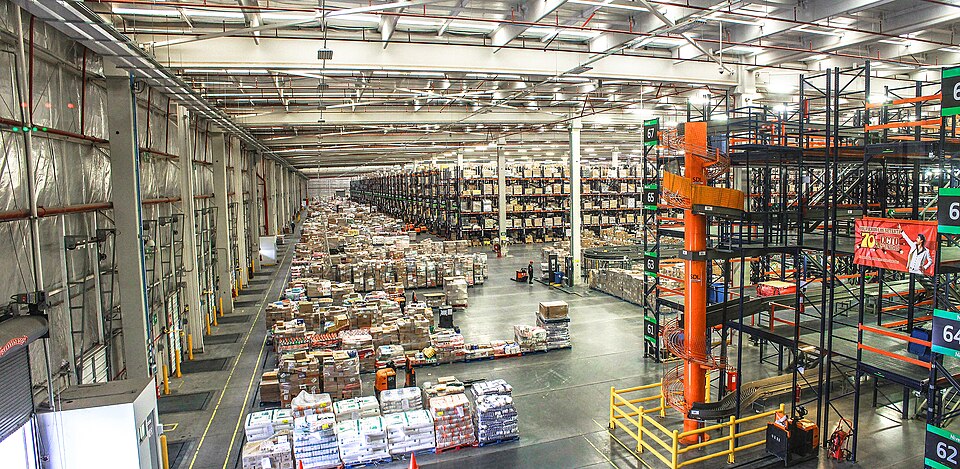Warehouse in a supply chain (Image: Rsherwin, CC BY-SA 4.0, via Wikimedia Commons)