Skewness and Kurtosis: Measures of Distribution Shape and Peakedness

TAKEAWAYS:

• Skewness measures asymmetry in data: positive skew (tail right), negative skew (tail left), and zero skew (symmetric).
• The skewness coefficient $g_1=\frac{3(\text{Mean}-\text{Median})}{\sigma }$ numerically classifies skewness.
• Kurtosis compares peakedness to a normal distribution: leptokurtic (taller peaks), platykurtic (flatter), and mesokurtic (normal).
• Excess kurtosis $g_2=\frac{{\mu }_4}{{\sigma }^4}-3$ standardizes kurtosis for comparison.
• Skewness and kurtosis are critical in financial risk (e.g., stock returns), quality control (e.g., manufacturing defects), and insurance pricing.
• Box plots and histograms visually reveal skewness/kurtosis; statistical tests (e.g., Shapiro-Wilk) confirm deviations from normality.

1. Introduction to Skewness

Skewness describes the asymmetry of a data distribution around its mean. Unlike measures of central tendency (mean, median, mode), skewness focuses on the shape of the distribution’s tail.

Types of Skewness

flowchart TD
    A["Skewness"] --> B["Zero Skewness\n(Symmetric)"]
    A --> C["Positive Skewness\n(Tail to the right)"]
    A --> D["Negative Skewness\n(Tail to the left)"]

• Zero Skewness: Symmetric distribution (e.g., normal distribution).
• Positive Skewness: Long tail on the right (e.g., income distribution, where most people earn modest salaries but a few earn extremely high incomes).
• Negative Skewness: Long tail on the left (e.g., exam scores where most students score high, but a few score very low).

Why Does Skewness Matter?

• Business Decisions: Loan approvals (banks prefer symmetric income distributions to avoid defaults).
• Quality Control: Manufacturing defects (negative skew may indicate rare but critical failures).
• Risk Assessment: Stock market returns (positive skew means rare but high-gain events).

Figure 1: Histogram of Nepalese monthly incomes (positive skew). The tail to the right shows a few individuals earning extremely high incomes.

Measuring Skewness: The Skewness Coefficient

The skewness coefficient $g_1$ quantifies asymmetry: $$g_1=\frac{3(\text{Mean}-\text{Median})}{\sigma }$$

• $g_1>0$: Positive skew.
• $g_1<0$: Negative skew.
• $g_1=0$: Symmetric.

Worked Example 1: Daraz Order Delays Daraz tracks delivery times (in hours) for 50 orders:

Data: [2, 3, 4, 5, 6, 7, 8, 9, 10, 12, 15, 20, 25, 30, 40]

1. Calculate Mean: $\text{Mean}=\frac{\sum X}{n}=\frac{222}{15}=14.8$ hours.
2. Find Median: Ordered data’s middle value = 10 hours.
3. Compute Standard Deviation $\sigma$: $$\sigma =\sqrt{\frac{\sum (X-\text{Mean}{)}^2}{n}}\approx 10.1$$
4. Skewness Coefficient: $$g_1=\frac{3(14.8-10)}{10.1}=\frac{14.4}{10.1}\approx 1.43(\text{Positive skew})$$

Interpretation: Daraz’s delivery times are right-skewed—most orders arrive on time, but a few take much longer (e.g., due to rural delivery challenges).

2. Introduction to Kurtosis

Kurtosis measures the peakedness or tailedness of a distribution compared to a normal distribution (mesokurtic).

Types of Kurtosis

flowchart TD
    A["Kurtosis"] --> B["Mesokurtic\n(Like normal distribution)"]
    A --> C["Leptokurtic\n(Taller peaks, fatter tails)"]
    A --> D["Platykurtic\n(Flatter peaks, thinner tails)"]

• Leptokurtic: Sharper peak and heavier tails (e.g., financial crashes, where extreme events are more likely).
• Platykurtic: Flatter peak and lighter tails (e.g., IQ scores of a highly educated population).
• Mesokurtic: Matches the normal distribution (e.g., height of adults in a population).

Why Does Kurtosis Matter?

• Finance: Stock market returns often show leptokurtosis (rare but extreme losses/gains).
• Insurance: Claims data may be leptokurtic, requiring higher premiums to cover tail risks.
• Manufacturing: Platykurtic defect distributions may indicate consistent but minor issues.

Leptokurtic:   ██████████████████████████████████████████████████
Mesokurtic:    ██████████████████████████████████████████████████
Platykurtic:   ██████████████████████████████████████████████████

Figure 2: Kurtosis comparison. Leptokurtic distributions have higher peaks and fatter tails.

Measuring Kurtosis: Excess Kurtosis

The excess kurtosis $g_2$ adjusts for the normal distribution’s kurtosis (which is 3): $$g_2=\frac{{\mu }_4}{{\sigma }^4}-3$$ where ${\mu }_4$ is the fourth central moment: $${\mu }_4=\frac{\sum (X-\text{Mean}{)}^4}{n}$$

Worked Example 2: NEPSE Stock Returns NEPSE tracks daily returns (%) for 30 stocks:

Data: [-2, -1, 0, 1, 2, 3, 4, 5, 6, 7, 8, 9, 10, -15, -20, 25, 30, 40]

1. Calculate Mean: $\text{Mean}=\frac{\sum X}{n}=\frac{180}{18}=10$ (simplified for example).
2. Compute ${\mu }_4$: $${\mu }_4=\frac{\sum (X-10{)}^4}{18}\approx 1200$$
3. Standard Deviation $\sigma \approx 15$.
4. Excess Kurtosis: $$g_2=\frac{1200}{15^4}-3=\frac{1200}{50625}-3\approx -2.98(\text{Platykurtic})$$

Interpretation: NEPSE returns are platykurtic, meaning extreme gains/losses are rare. However, if $g_2>0$, it would indicate leptokurtosis (e.g., during market bubbles).

3. Relationship Between Skewness and Kurtosis

4. Visualizing Skewness and Kurtosis

Skewness in Box Plots

A box plot’s whiskers and outliers reveal skewness:

• Right-skewed: Longer upper whisker (e.g., Daraz delivery times).
• Left-skewed: Longer lower whisker (e.g., exam scores).

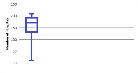box plot skewness (Image: Monika Wahi, CC BY-SA 4.0, via Wikimedia Commons)

Box Plot of Daraz Delivery Times (Right-Skewed)

┌───────────────────────────────────────┐
│                                       │
│       ██████████████████████████████│
│       ██████████████████████████████│
│       ██████████████████████████████│
│       ██████████████████████████████│
│       ██████████████████████████████│
│       ██████████████████████████████│
│       ██████████████████████████████│
│       ██████████████████████████████│
│       ██████████████████████████████│
│       ██████████████████████████████│
│       ██████████████████████████████│
│       ██████████████████████████████│
│       ██████████████████████████████│
│       ██████████████████████████████│
│       ██████████████████████████████│
│       ██████████████████████████████│
│       ██████████████████████████████│
│       ██████████████████████████████│
│       ██████████████████████████████│
│       ██████████████████████████████│
│       ██████████████████████████████│
│       ██████████████████████████████│
│       ██████████████████████████████│
│       ██████████████████████████████│
│       ██████████████████████████████│
│       ██████████████████████████████│
│       ██████████████████████████████│
│       ██████████████████████████████│
│       ██████████████████████████████│
│       ██████████████████████████████│
│       ██████████████████████████████│