Economics for BusinessUnit 410 min read
Production Functions, Returns, Efficiency & Tech Change
Unit 4 of Economics for Business explains how firms combine inputs (land, labor, capital) to produce outputs, analyzes short-run vs. long-run production decisions, and evaluates technological progress—with real-world examples from Nepal’s garment factories, Daraz logistics, and Ncell’s network expansion.
Core Concepts: What is Production?
Production is the process of combining inputs (factors of production) to create outputs (goods/services). Businesses aim to maximize output while minimizing costs. The theory of production studies how firms make these decisions under different conditions.
Key Inputs (Factors of Production)
Every production process relies on four fundamental inputs:
| Factor | Description | Example in Nepal |
|---|---|---|
| Land | Natural resources (land, water, minerals) | Tea gardens in Ilam, hydropower sites in Dolpo, Daraz’s warehouses in Kathmandu. |
| Labor | Human effort (skilled/unskilled workers) | Garment workers in Chitwan, Ncell customer service agents, Pathao delivery riders. |
| Capital | Man-made tools/machinery (buildings, equipment) | Khalti’s servers, NTC’s fiber-optic cables, Daraz’s automated sorting robots. |
| Entrepreneurship | Risk-taking, innovation, management skills | Founders of F1Soft (Nepal’s first software company), Nepal Investment Bank. |
Production Functions: How Inputs Become Output
A production function shows the maximum output a firm can produce from given inputs. Mathematically: Where:
- = Quantity of output
- = Labor
- = Capital
- Tech = Technology level
Short-Run vs. Long-Run Production
| Aspect | Short-Run | Long-Run |
|---|---|---|
| Time Frame | At least one input is fixed (e.g., factory size). | All inputs are variable (can be adjusted). |
| Example | A Daraz warehouse hiring more workers but using the same space. | Ncell building a new 5G tower and training staff. |
| Key Focus | How to use variable inputs (labor, raw materials) efficiently. | Optimal combination of all inputs (e.g., automation vs. labor). |
Stages of Production and Returns
When a firm increases only one variable input (e.g., labor) while keeping others fixed, it moves through three stages of production:
1. Law of Variable Proportions (Diminishing Returns)
As more of a variable input (e.g., labor) is added to a fixed input (e.g., machinery), marginal product (additional output per unit of input) eventually falls.
graph TD
    A["Stage 1: Increasing Returns"] --> B["Marginal Product Rising"]
    B --> C["More workers = More output per worker"]
    C --> D["Example: First 5 workers in a factory"]
    D --> E["Output: 100 units"]
    F["Stage 2: Diminishing Returns"] --> G["Marginal Product Falls"]
    G --> H["Adding more workers increases output, but at a slower rate"]
    H --> I["Example: 10th worker adds only 10 units"]
    I --> J["Output: 150 units (total)"]
    K["Stage 3: Negative Returns"] --> L["Marginal Product Negative"]
    L --> M["Too many workers = Output decreases"]
    M --> N["Example: 20th worker breaks equipment"]
    N --> O["Output: 140 units (total)"]
Worked Example: A Garment Factory in Chitwan
- Fixed Input: 10 sewing machines.
- Variable Input: Labor (workers).
- Output (shirts per day):
- 1 worker → 50 shirts
- 5 workers → 200 shirts (Stage 1: Increasing returns)
- 10 workers → 350 shirts (Stage 2: Diminishing returns)
- 15 workers → 330 shirts (Stage 3: Negative returns—machines jam!)
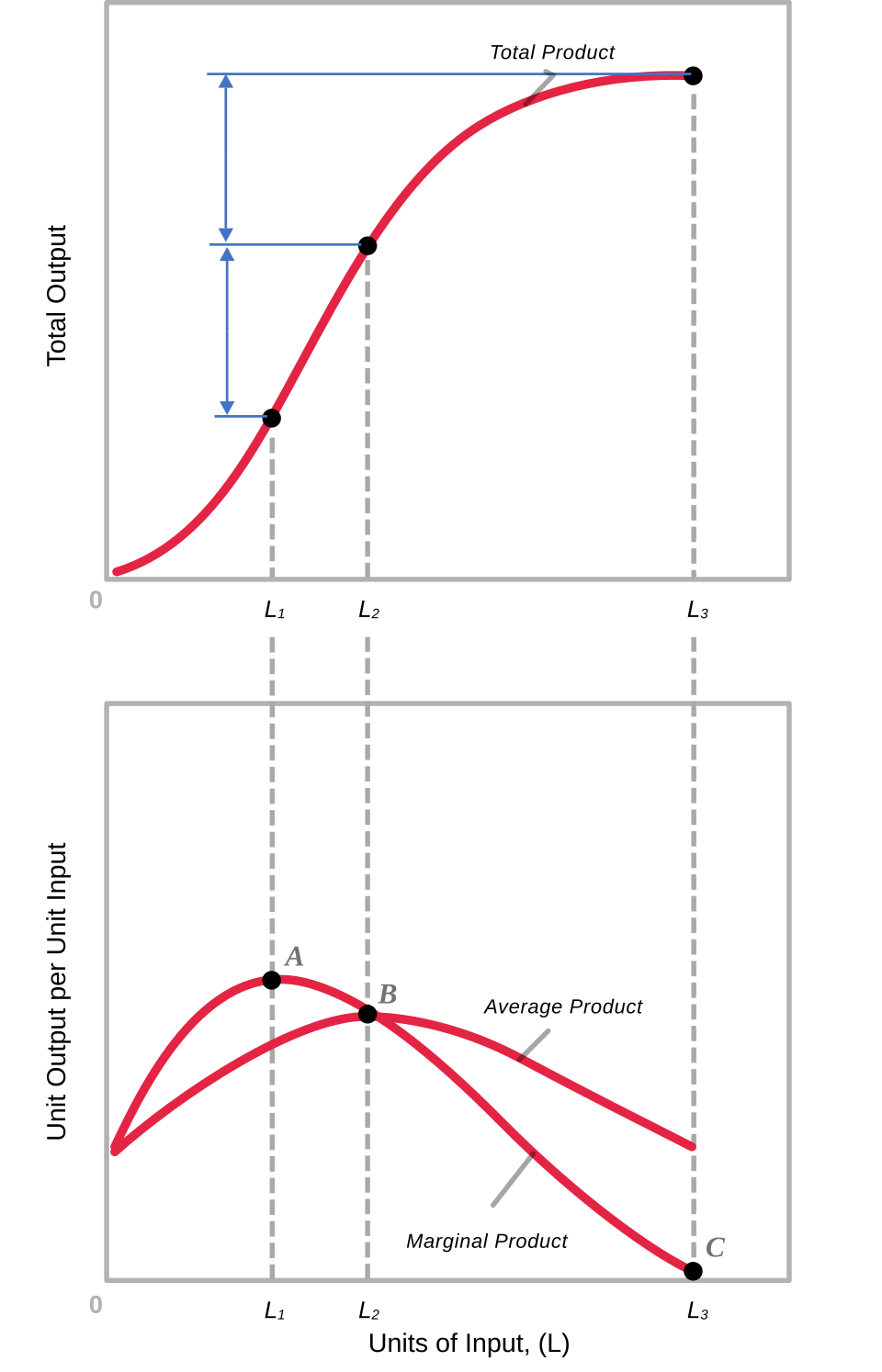 A curve showing total product (TP), average product (AP), and marginal product (MP) for labor in the Chitwan factory example, with Stage 1, 2, and 3 labeled. (Image: Vectorization: Alhadis, CC BY-SA 4.0, via Wikimedia Commons)
Types of Production Functions
1. Linear Production Function
Output increases proportionally with inputs. Example: A Nepal Rastra Bank printing press where each worker adds the same number of notes.
2. Cobb-Douglas Production Function
Most common in real-world modeling: Where:
- = Total Factor Productivity (tech efficiency)
- = Output elasticity (how sensitive Q is to inputs)
Example: Ncell’s Network Expansion If , increasing labor by 10% raises output by 6%, while adding capital raises it by 4%.
Efficiency and Optimal Input Combination
Firms aim for technical efficiency (maximum output from given inputs) and economic efficiency (minimum cost for desired output).
Isoquants and Isocosts
- Isoquant: Curve showing all input combinations yielding the same output.
- Isocost: Line showing all input combinations with the same cost.
graph LR
    A["Isoquant (Q=100 units)"] --> B["More Labor, Less Capital"]
    A --> C["Less Labor, More Capital"]
    D["Isocost (Cost = Rs. 50,000)"] --> E["High Labor Cost"]
    D --> F["High Capital Cost"]
    G["Optimal Point"] --> H["Tangency of Isoquant & Isocost"]
    H --> I["MRTS = Price Ratio"]
Worked Example: Daraz’s Warehouse
- Output Goal: 1,000 orders/day.
- Inputs:
- Labor cost = Rs. 500/worker/day
- Capital cost = Rs. 1,000/machine/day
- Optimal Combination: 10 workers + 5 machines (lowest cost for 1,000 orders).
Returns to Scale
What happens when all inputs are increased proportionally?
| Type | Description | Example |
|---|---|---|
| Increasing RTS | Doubling inputs > doubles output. | Nepal Investment Bank expanding branches and staff sees loan growth > 100%. |
| Constant RTS | Doubling inputs = doubles output. | A tea factory where scaling up workers and machinery exactly doubles tea output. |
| Decreasing RTS | Doubling inputs < doubles output (due to coordination issues). | Khalti adding too many servers may slow down due to network congestion. |
Technological Progress and Innovation
Technological change shifts the production function upward, allowing more output from the same inputs.
Types of Tech Progress
- Labor-Augmenting: Improves worker productivity (e.g., Ncell’s 5G upgrade).
- Capital-Augmenting: Better machinery (e.g., Daraz’s automated sorting robots).
- Neutral: Improves both labor and capital equally (e.g., Nepal Rastra Bank’s digital banking software).
Real-World Impact in Nepal:
- Pathao’s AI routing reduced delivery time by 30% (labor-augmenting).
- Nepal Stock Exchange (NEPSE) automated trading (capital-augmenting).
- Khalti’s blockchain improved transaction speed (neutral).
In the Real World
Daraz’s Logistics Hubs
- Idea Used: Isoquant optimization (balancing labor and automated sorting machines).
- How? Daraz’s Rs. 200 million warehouse in Kathmandu uses 60% robots and 40% workers to handle 50,000 orders/day at minimal cost.
Ncell’s Network Expansion
- Idea Used: Cobb-Douglas function to model tower placement.
- How? Ncell’s 5G rollout followed , prioritizing labor-trained technicians over just adding towers.
Nepal’s Garment Industry (Chitwan)
- Idea Used: Law of Diminishing Returns.
- How? Factories hire up to 12 workers per machine—beyond that, output drops due to congestion.
Exam Tip
What Examiners Look For
- Diagrams > Words: Always draw isoquants, TP/MP/AP curves, and PPC with labels. A well-labeled graph can fetch 5+ marks.
- Real-World Links: Relate Daraz, Ncell, or NEPSE to concepts like returns to scale or technological progress.
- Maths + Words: For Cobb-Douglas, show both the equation and interpretation (e.g., "If , labor is more important than capital").
- Short-Run vs. Long-Run: Always clarify which stage (fixed/variable inputs) you’re analyzing.
- Common Mistakes to Avoid:
- Confusing marginal product (additional output) with average product (output per worker).
- Forgetting Stage 3 (negative returns) in production stages.
- Ignoring technological change in long-run analysis.
Sample Exam Question & Answer Structure
Question: "Explain the law of variable proportions with a numerical example from Nepal’s garment industry. How does this relate to a firm’s hiring decisions?"
Model Answer:
- Definition: Law of variable proportions states that as one variable input (labor) increases while others (capital) are fixed, marginal product first rises, then falls, then becomes negative.
- Numerical Example (using the Chitwan factory table above).
- Graph: Draw TP, AP, MP curves with Stage 1, 2, 3 labeled.
- Firm’s Decision:
- Stage 1 (1–5 workers): Hire more—output rises efficiently.
- Stage 2 (6–10 workers): Still hire, but at diminishing returns.
- Stage 3 (11+ workers): Stop hiring—output falls.
- Real-World Link: "Like Fashion Place factories, firms must avoid over-hiring beyond Stage 2 to prevent losses."
Final Checklist Before Exam ✅ Can you draw and label TP/MP/AP curves? ✅ Do you know Cobb-Douglas and how to interpret exponents? ✅ Can you explain isoquants/isocosts with a Daraz/Ncell example? ✅ Do you compare short-run vs. long-run production? ✅ Can you calculate marginal product from a table?
Based on the TU BIM syllabus for Economics for Business (ECO206), unit 4.
Discussion
Loading…