Data Warehousing and Data MiningUnit 412 min read
Data Preprocessing: Cleaning, Integration, Transformation, Reduction
Unit 4 of Data Warehousing and Data Mining: covers the essential steps of preparing raw data for analysis, including handling missing values, outliers, data integration, transformation, and reduction techniques.
Key points
- Data preprocessing is the most time-consuming phase (up to 80%) of the data mining process.
- Missing values must be handled via deletion, imputation, or regression to prevent biased models.
- Data integration combines data from multiple sources, requiring resolution of schema conflicts and entity identity issues.
- Data transformation normalizes data (e.g., z-score, min-max) to ensure features are on comparable scales.
- Data reduction reduces dimensionality (PCA) or cardinality (sampling) to improve efficiency without losing significant information.
- Outlier detection is critical to prevent extreme values from skewing statistical measures like mean and standard deviation.
1. Introduction to Data Preprocessing
Data preprocessing is the process of transforming raw data into a clean, consistent, and useful format for data mining. In real-world scenarios, data is rarely "clean." It often contains missing values, noise, inconsistencies, and redundancies. If this data is fed directly into a data mining algorithm, the results will be inaccurate or misleading.
The primary goal is to improve data quality. High-quality data leads to high-quality models. The main tasks involved are:
- Data Cleaning: Handling missing values, noisy data, and inconsistent data.
- Data Integration: Combining data from multiple sources.
- Data Transformation: Converting data into forms suitable for mining.
- Data Reduction: Producing a reduced representation of the data that is much smaller in size but still maintains a high level of fidelity.
flowchart LR
    A["Raw Data Sources"] --> B["Data Cleaning"]
    B --> C["Data Integration"]
    C --> D["Data Transformation"]
    D --> E["Data Reduction"]
    E --> F["Data Mining"]
    F --> G["Knowledge Discovery"]
2. Data Cleaning
Data cleaning involves detecting and correcting (or deleting) errors and inconsistencies in the data.
2.1 Handling Missing Values
Missing values are common in real-world databases. If not handled, they can cause errors in algorithms that require complete records.
Strategies:
- Ignore the tuple: Only useful if the tuple is missing values for multiple attributes and the majority of the data is missing.
- Manual entry: Tedious and time-consuming; only feasible for small datasets.
- Global constant: Fill all missing values with a constant like
?,Unknown, or0. - Attribute mean/median: Fill with the mean or median of the known values for that attribute.
- Most probable value: Use regression or a decision tree/induction algorithm to infer the missing value from other attributes.
Worked Example: Imputation by Mean
Consider a dataset of student marks in Mathematics.
Data: 50, 60, ?, 70, 80
- Sum of known values:
- Count of known values:
- Mean:
- Replace
?with65. New Data:50, 60, 65, 70, 80
2.2 Handling Noisy Data
Noisy data contains errors or deviations from the expected value.
Smoothing Techniques:
- Binning:
- Sort the data.
- Partition into bins of equal depth (number of records) or equal width (value range).
- Smooth by bin means, bin midpoints, or bin boundaries.
- Regression: Fit the data to a function (e.g., linear regression line).
- Clustering: Group similar data points together; points far from the cluster center are considered noise/outliers.
Worked Example: Binning by Bin Means
Data: 4, 8, 15, 16, 23, 42, 50, 55
- Sort:
4, 8, 15, 16, 23, 42, 50, 55 - Partition: Let bin depth = 2.
- Bin 1:
4, 8 - Bin 2:
15, 16 - Bin 3:
23, 42 - Bin 4:
50, 55
- Bin 1:
- Calculate Bin Means:
- Mean 1:
- Mean 2:
- Mean 3:
- Mean 4:
- Smooth: Replace values in each bin with the bin mean.
- Result:
6, 6, 15.5, 15.5, 32.5, 32.5, 52.5, 52.5
- Result:
2.3 Handling Outliers
Outliers are data points that deviate significantly from the rest of the data. They can be errors or rare events.
Detection Methods:
- Box Plot:
- Calculate Q1 (25th percentile), Q2 (Median), Q3 (75th percentile).
- Interquartile Range (IQR) = .
- Lower Bound:
- Upper Bound:
- Any value outside these bounds is an outlier.
Worked Example: Box Plot Detection
Data: 10, 12, 14, 15, 16, 18, 100
- Sorted:
10, 12, 14, 15, 16, 18, 100 - Median (Q2) = 15
- Lower Half:
10, 12, 14-> Q1 = 12 - Upper Half:
16, 18, 100-> Q3 = 18 - IQR =
- Lower Bound =
- Upper Bound =
- Check:
100is greater than27. - Conclusion:
100is an outlier.
3. Data Integration
Data integration involves combining data from multiple heterogeneous sources into a coherent data store.
Key Issues:
- Redundancy: The same real-world entity may be represented differently in different sources (e.g., "Nepal" vs. "NPL" vs. "NP").
- Inconsistency: Conflicting information about the same real-world entity (e.g., two sources give different phone numbers for the same customer).
- Schema Integration: Mapping concepts from different schemas to a global schema.
Resolution Strategies:
- Entity Resolution: Determining whether two records refer to the same real-world entity.
- Conflict Resolution: Using rules or statistical methods to decide which value is correct (e.g., most recent timestamp, majority vote).
4. Data Transformation
Data transformation involves normalizing or aggregating data.
4.1 Normalization
Normalization scales data to a specific range to prevent attributes with larger ranges from dominating the distance calculations in algorithms like K-Means or K-NN.
Common Techniques:
Min-Max Normalization: Maps values to a range .
Z-Score Standardization: Uses mean and standard deviation. Where is the mean and is the standard deviation.
Decimal Scaling: Moves the decimal point of values. Where is the smallest number such that .
Worked Example: Min-Max Normalization Attribute: Age. Range: . Target Range: . Value to normalize: .
Worked Example: Z-Score
Data: 4, 8, 6, 5, 3, 9
- Mean ():
- Standard Deviation (): Calculations: Sum = Variance =
- Normalize :
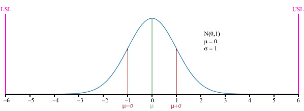 Illustration of z-score standardization showing how data points relate to the mean and standard deviation. (Image: Jayen466, Fleshgrinder, Public domain, via Wikimedia Commons)
4.2 Aggregation
Aggregation involves summarizing data at a higher level of abstraction.
- Example: Aggregating daily sales data into monthly sales data.
- This reduces the volume of data and can reveal trends that are hidden in raw data.
5. Data Reduction
Data reduction aims to produce a smaller but representative version of the original dataset.
5.1 Dimensionality Reduction
Reducing the number of attributes (features).
Principal Component Analysis (PCA):
- Transforms correlated variables into a set of uncorrelated variables called principal components.
- The first principal component explains the most variance in the data.
- Useful for visualization and noise reduction.
Feature Selection:
- Selecting a subset of relevant features.
- Methods: Filter (statistical tests), Wrapper (model-based), Embedded (during model training).
5.2 Cardinality Reduction
Reducing the number of records (rows).
Sampling:
- Simple Random Sampling: Each tuple has an equal chance of being selected.
- Stratified Sampling: The dataset is divided into strata (groups), and samples are drawn from each stratum proportionally. This ensures representation of all classes.
Histograms:
- Approximate the data distribution using bins.
Clustering:
- Represent the data by cluster centers.
Comparison Table: Data Reduction Techniques
| Technique | Goal | Method | Use Case |
|---|---|---|---|
| PCA | Reduce Dimensions | Linear transformation | High-dimensional data, visualization |
| Feature Selection | Reduce Dimensions | Select best features | When interpretability is needed |
| Sampling | Reduce Cardinality | Random/Stratified selection | Large datasets, initial exploration |
| Histograms | Reduce Cardinality | Binning | Distribution analysis |
6. In the real world
Data preprocessing is the backbone of modern data-driven businesses in Nepal and globally.
eSewa and Khalti (Financial Fintech):
- Concept: Data Cleaning and Outlier Detection.
- Application: eSewa processes millions of transactions daily. A sudden spike in transaction volume from a single user account might be flagged as an outlier. The system uses statistical thresholds (like the Z-score method) to detect potential fraud. If a user who usually spends Rs. 500 suddenly spends Rs. 50,000, the system flags it for manual review. This prevents financial loss and ensures data integrity for risk analysis models.
Daraz (E-commerce):
- Concept: Data Integration and Entity Resolution.
- Application: Daraz aggregates data from multiple sellers, logistics partners, and payment gateways. A customer's order might be recorded in the seller's system as "Kathmandu, Nepal" and in the logistics system as "KTM, NP". Data integration algorithms resolve these entity identity issues to ensure the customer receives accurate tracking updates. Without this, the "single view of the customer" would be fragmented, leading to poor customer service and inaccurate inventory forecasting.
Ncell (Telecommunications):
- Concept: Data Transformation (Normalization).
- Application: Ncell analyzes customer usage patterns to predict churn (customers leaving the service). One attribute might be "Monthly Bill" (range: Rs. 100 - Rs. 10,000) and another "Call Minutes" (range: 0 - 1000). If not normalized, the "Monthly Bill" would dominate the distance calculations in clustering algorithms because its range is larger. Ncell uses Min-Max normalization to scale both attributes to [0, 1], ensuring that both billing and usage patterns contribute equally to identifying at-risk customers.
7. Exam tip
In TU and PU exams, Unit 4 is frequently tested through numerical problems and conceptual comparisons.
- Numerical Focus: Be prepared to calculate Bin Means, Z-Scores, and Min-Max Normalization. Show every step of the calculation. For Box Plots, explicitly state Q1, Q3, IQR, and the bounds.
- Conceptual Focus: Differentiate between Data Cleaning (fixing errors) and Data Reduction (shrinking size). Understand the difference between Filter and Wrapper feature selection.
- Diagrams: If asked about the Data Preprocessing pipeline, draw a clear flowchart showing the sequence: Cleaning -> Integration -> Transformation -> Reduction.
- Common Trap: Do not confuse Outliers (extreme values) with Missing Values (absent data). They require different handling strategies.
In the real world
eSewa (Nepal) uses data cleaning to handle missing or inconsistent transaction records before generating financial reports. For example, if a user’s phone number is missing in their profile, eSewa’s system fills it with the last known valid number (global constant method) to ensure smooth transactions.
Pathao (Nepal) applies normalization to rider ratings (1–5 stars) before calculating driver performance scores. Ratings are scaled to a 0–1 range to ensure fairness in comparisons across different cities.
Nepal Electricity Authority (NEA) performs outlier detection on electricity consumption data to identify fraudulent usage. For instance, a household consuming 1000 units in a month (while neighbors average 100–200) is flagged as an outlier for investigation.
Based on the TU BIM syllabus for Data Warehousing and Data Mining (IT274), unit 4.
Discussion
Loading…