Partial Derivatives – definitions, first & higher order, gradient, tangent plane, chain rule

1. What is a Partial Derivative?

For a function of two variables $f(x,y)$ the partial derivative with respect to $x$ is the ordinary derivative of $f$ when $y$ is treated as a constant:

$$\frac{\partial f}{\partial x}(x_0,y_0)=\underset{h\to 0}{\lim }\frac{f(x_0+h,y_0)-f(x_0,y_0)}{h}.$$

Similarly for $y$:

$$\frac{\partial f}{\partial y}(x_0,y_0)=\underset{k\to 0}{\lim }\frac{f(x_0,y_0+k)-f(x_0,y_0)}{k}.$$

These are the slopes of the surface $z=f(x,y)$ along the coordinate directions.

The contour lines are curves of constant $z$. The spacing of the lines is tighter where the partial derivative with respect to the corresponding variable is larger.

2. Computing First‑Order Partial Derivatives

Treat all other variables as constants and differentiate normally.

Worked Example 1 – From the past exam:

Find $\frac{\partial f}{\partial x}$ and $\frac{\partial f}{\partial y}$ at $(4,-5)$ for

$$f(x,y)=x^2+3xy+y-1.$$

Solution

1. $\frac{\partial f}{\partial x}=2x+3y$ (differentiate w.r.t. $x$, $y$ constant).
2. $\frac{\partial f}{\partial y}=3x+1$ (differentiate w.r.t. $y$, $x$ constant).

Evaluate at $(4,-5)$:

$$\frac{\partial f}{\partial x}(4,-5)=2(4)+3(-5)=8-15=-7,$$ $$\frac{\partial f}{\partial y}(4,-5)=3(4)+1=12+1=13.$$

Thus the gradient at the point is $\nabla f(4,-5)=⟨-7,13⟩$.

3. Second‑Order and Mixed Partial Derivatives

Higher‑order partials are obtained by differentiating a first‑order partial again.

3.1 Notation

$$f_{xx}=\frac{{\partial }^{2}f}{\partial x^2},f_{yy}=\frac{{\partial }^{2}f}{\partial y^2},f_{xy}=\frac{{\partial }^{2}f}{\partial x\partial y},f_{yx}=\frac{{\partial }^{2}f}{\partial y\partial x}.$$

3.2 Clairaut’s (Schwarz) Theorem

If the mixed partials $f_{xy}$ and $f_{yx}$ are continuous on a neighbourhood of a point, then

$$f_{xy}=f_{yx}.$$

3.3 Worked Example 2 – Second‑order derivatives

Find all second‑order partial derivatives of

$$f(x,y)=x^4-5x^3{y}^2+7x^2{y}^3+4x{y}^5.$$

Solution

First‑order partials:

$$\begin{array}{rl}{f}_x& =4x^3-15x^2{y}^2+14x{y}^3+4y^5,\\ f_y& =-10x^{3}y+21x^2{y}^2+20x{y}^4.\end{array}$$

Second‑order:

$$\begin{array}{rl}{f}_{xx}& =12x^2-30x{y}^2+14y^3,\\ f_{yy}& =-10x^3+42x^{2}y+80x{y}^3,\\ f_{xy}& =\frac{\partial }{\partial y}{f}_x=-30x^{2}y+42x{y}^2+20y^4,\\ f_{yx}& =\frac{\partial }{\partial x}{f}_y=-30x^{2}y+42x{y}^2+20y^4.\end{array}$$

Since $f_{xy}=f_{yx}$ everywhere, Clairaut’s condition is satisfied.

The surface plot shows the rapid growth in the positive octant, illustrating why the mixed derivatives are identical.

4. The Gradient Vector

The gradient of $f$ is the vector of its first‑order partials:

$$\nabla f(x,y)=⟨\frac{\partial f}{\partial x},\frac{\partial f}{\partial y}⟩.$$

Properties:

The arrows illustrate how the gradient changes across the plane.

5. Tangent Plane and Linear Approximation

For a differentiable surface $z=f(x,y)$ at $(x_0,y_0)$ the tangent plane is

$$z=f(x_0,y_0)+f_x(x_0,y_0)(x-x_0)+f_y(x_0,y_0)(y-y_0).$$

The linear approximation (or first‑order Taylor polynomial) uses this plane to estimate nearby values:

$$L(x,y)=f(x_0,y_0)+\nabla f(x_0,y_0)\cdot ⟨x-x_0,y-y_0⟩.$$

Worked Example 3 – Tangent plane for the function in Example 1 at $(4,-5)$.

We already have $f(4,-5)=4^2+3\cdot 4\cdot (-5)+(-5)-1=16-60-5-1=-50$.
Partial derivatives at the point: $f_x=-7$, $f_y=13$.

Hence

$$z=-50-7(x-4)+13(y+5).$$

Simplified:

$$z=-7x+13y+2.$$

The picture shows the surface (blue) and the red tangent plane intersecting at the point.

6. Multivariable Chain Rule

If $z=f(x,y)$ where $x=g(t)$ and $y=h(t)$ are functions of a single parameter $t$, then

$$\frac{dz}{dt}=f_x\frac{dx}{dt}+f_y\frac{dy}{dt}.$$

For a composition with two parameters, e.g. $x=g(s,t)$, $y=h(s,t)$,

$$\begin{array}{rl}\frac{\partial z}{\partial s}& =f_x\frac{\partial x}{\partial s}+f_y\frac{\partial y}{\partial s},\\ \frac{\partial z}{\partial t}& =f_x\frac{\partial x}{\partial t}+f_y\frac{\partial y}{\partial t}.\end{array}$$

flowchart LR
    A["z = f(x,y)"] --> B["x = g(s,t)"]
    A --> C["y = h(s,t)"]
    B --> D["∂z/∂s = fₓ·∂x/∂s + fᵧ·∂y/∂s"]
    C --> D
    B --> E["∂z/∂t = fₓ·∂x/∂t + fᵧ·∂y/∂t"]
    C --> E

The diagram summarises the flow of derivatives.

7. Applications of Partial Derivatives

8. In the real world

1. eSewa payment gateway – The fee‑structure function $F(t,c)=a{t}^2+bc$ (where $t$ = transaction amount, $c$ = number of concurrent users) uses $\partial F/\partial t$ to decide how the fee changes when transaction size grows, ensuring the platform remains profitable while keeping fees competitive.

2. Daraz order‑fulfilment – The expected delivery time $D(x,y)=\alpha x^2+\beta y$ (with $x$ = number of orders in a zone, $y$ = distance to warehouse) is optimised by setting $\partial D/\partial x=0$ and $\partial D/\partial y=0$ to allocate couriers efficiently.

3. NEPSE stock‑price model – A simple two‑factor model $P(r,v)=k_1{r}^2+k_{2}v$ (where $r$ = interest rate, $v$ = market volatility) uses the gradient $\nabla P$ to gauge which factor influences price more on a given day, guiding traders’ decisions.

Worked real‑world tie‑in: A Nepali bank wants to maximise its monthly revenue from personal loans. The revenue model is

$$R(r,L)=L\cdot r-0.001L^2,$$

where $r$ is the interest rate (in %) and $L$ is the total loan amount (in million NPR).

• $\frac{\partial R}{\partial r}=L$ tells the bank that each additional 1 % point in rate adds revenue equal to the current loan portfolio.
• $\frac{\partial R}{\partial L}=r-0.002L$. Setting this to zero gives the optimal loan amount for a chosen rate: $L^{\ast }=\frac{r}{0.002}$.

If the bank currently offers $r=12\%$, the optimal loan amount is $L^{\ast }=\frac{12}{0.002}=6000$ million NPR. The bank can therefore adjust marketing to target this loan volume.

9. Summary Table

Exam tip

• Memorise the notation: $\partial$ for partials, subscripts for order, and the gradient arrow $\nabla$.
• Always state the variable you are holding constant before differentiating; this avoids sign errors.
• For mixed partials, write both $f_{xy}$ and $f_{yx}$ and check continuity; most exam functions are polynomials, so equality holds automatically.
• When a question asks for the tangent plane, plug the point into the original function first, then compute the two first‑order partials at that point and substitute into the plane formula.
• Partial‑derivative chain‑rule problems are scored high if you draw a quick mermaid‑style flow (as shown above) to keep track of each inner derivative.
• Practice linear approximation: rewrite the answer as $L(x,y)$ and compare with the exact value to see the error magnitude – a common short‑answer check.

Good luck!

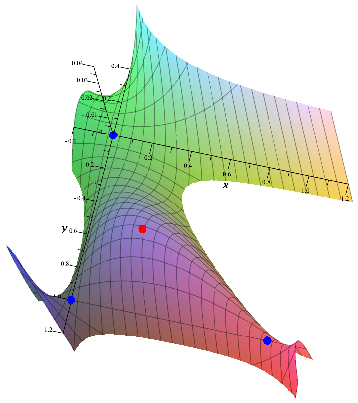3‑D surface of a two‑variable polynomial (Image: Kmhkmh, CC BY 3.0, via Wikimedia Commons)