Interpolation & Curve Fitting: Methods, Formulas & Applications

TAKEAWAYS:

• Interpolation estimates unknown values between known data points using polynomials (Lagrange, Newton), while curve fitting finds the best-fit function (least squares) for noisy data.
• Lagrange’s formula constructs a unique polynomial through $n+1$ points but becomes computationally expensive for large $n$.
• Newton’s divided differences builds polynomials incrementally (forward/backward) and is efficient for unevenly spaced data.
• Least squares minimizes error for overdetermined systems (more data points than parameters) and is used in regression analysis.
• Error bounds (e.g., $E(x)=\frac{f^{(n+1)}(\xi )}{(n+1)!}{\prod }_{i=0}^n(x-x_i)$) quantify interpolation accuracy.
• Applications span finance (stock trends), engineering (sensor calibration), and logistics (demand forecasting).

---

1. Introduction to Interpolation

Interpolation estimates a function’s value at an unmeasured point using known data points. It is widely used when:

• Exact solutions are impractical (e.g., experimental data).
• Closed-form functions are unavailable (e.g., stock prices).

Key Definitions

• Interpolation: Exact fitting through given points (error = 0 at $x_i$).
• Extrapolation: Predicting values outside the data range (higher error risk).
• Polynomial Interpolation: Uses polynomials of degree $n$ for $n+1$ points.

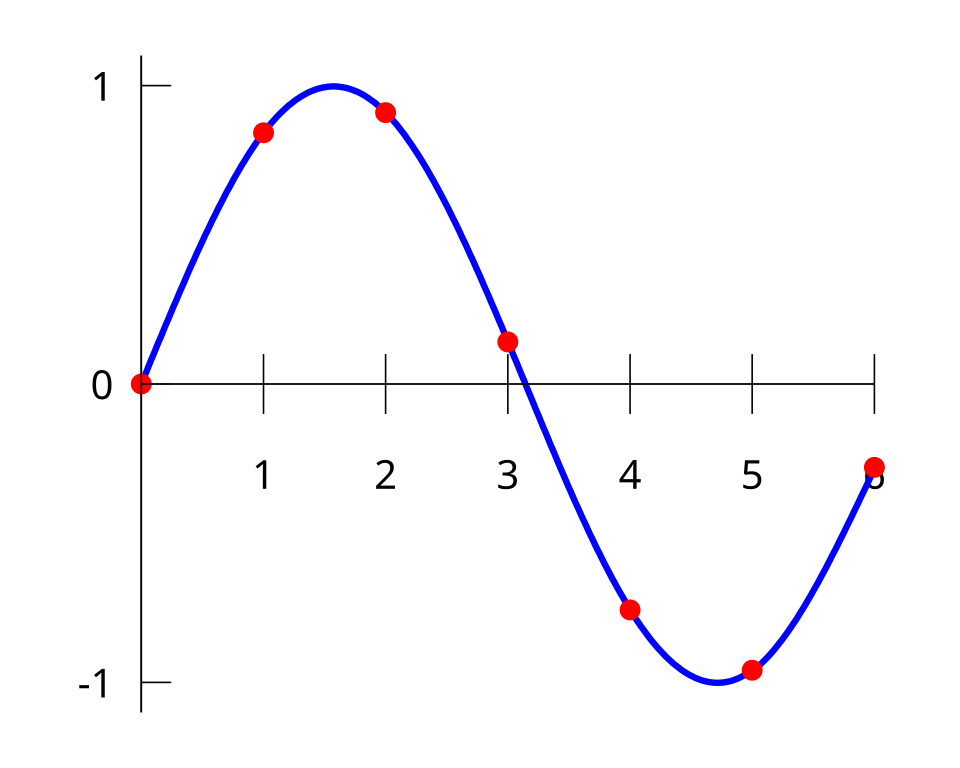
Visual: Data Points and Interpolation

Example 1.1: Given $f(1)=2$, $f(2)=3$, $f(3)=5$, find $f(1.5)$ using linear interpolation. Solution: Linear interpolation formula: $$P(x)=y_i+\frac{y_{i+1}-y_i}{x_{i+1}-x_i}(x-x_i)$$ For $x=1.5$ (between $x_1=1$ and $x_2=2$): $$P(1.5)=2+\frac{3-2}{2-1}(1.5-1)=2+0.5=2.5$$ Answer: $f(1.5)\approx 2.5$.

---

2. Lagrange Interpolation

Lagrange’s method constructs a polynomial $P_n(x)$ that passes through all $n+1$ points exactly.

Formula

$$P_n(x)=\sum _{i=0}^n{y}_i{L}_i(x),L_i(x)=\prod _{\begin{array}{c}j=0\\ j\ne i\end{array}}^n\frac{x-x_j}{x_i-x_j}$$ Advantages:

• Simple to derive for small $n$.
• No need to compute divided differences.

Disadvantages:

• Computationally expensive for large $n$ (O$(n^2)$).
• Unstable for high-degree polynomials (Runge’s phenomenon).

Worked Example 2.1: Lagrange Interpolation

Given: $$\begin{array}{ccccc}x& 1& 2& 3& 4\\ y& 1& 4& 9& 16\end{array}$$ Find $P_3(x)$ and estimate $f(2.5)$.

Solution: $$P_3(x)=1\cdot \frac{(x-2)(x-3)(x-4)}{(1-2)(1-3)(1-4)}+4\cdot \frac{(x-1)(x-3)(x-4)}{(2-1)(2-3)(2-4)}+\cdots$$ Simplify each $L_i(x)$: $$L_0(x)=\frac{(x-2)(x-3)(x-4)}{-6},L_1(x)=\frac{(x-1)(x-3)(x-4)}{2},\text{etc.}$$ Combine terms: $$P_3(x)=x^3$$ Estimate at $x=2.5$: $$P_3(2.5)=(2.5{)}^3=15.625$$ Visual: Lagrange Basis Polynomials

---

3. Newton’s Divided Differences

Newton’s method builds the polynomial incrementally using divided differences, avoiding recomputation.

Divided Differences Table

For points $(x_0,y_0),\dots ,(x_n,y_n)$: $$\begin{array}{cccc}{x}_0& y_0& & \\ & f[x_0,x_1]& & \\ x_1& y_1& f[x_0,x_1,x_2]& \\ & f[x_1,x_2]& & \\ x_2& y_2& ⋮& \end{array}$$ Where: $$f[x_i,x_{i+1}]=\frac{y_{i+1}-y_i}{x_{i+1}-x_i},f[x_i,\dots ,x_{i+k}]=\frac{f[x_{i+1},\dots ,x_{i+k}]-f[x_i,\dots ,x_{i+k-1}]}{x_{i+k}-x_i}$$

Newton’s Polynomial

$$P_n(x)=f[x_0]+f[x_0,x_1](x-x_0)+f[x_0,x_1,x_2](x-x_0)(x-x_1)+\cdots$$

Worked Example 3.1: Newton’s Forward Interpolation

Given: $$\begin{array}{ccccc}x& 1& 3& 5& 7\\ y& 1& 4& 9& 16\end{array}$$ Find $f(4)$ using Newton’s forward formula.

Solution: Compute divided differences: $$\begin{array}{cccc}1& 1& & \\ & 1& 0.5& \\ 3& 4& & 0\\ & 1& 0& \\ 5& 9& & \\ & 1& & \\ 7& 16& & \end{array}$$ Newton’s polynomial: $$P_3(x)=1+1(x-1)+0.5(x-1)(x-3)+0(x-1)(x-3)(x-5)$$ Simplify: $$P_3(x)=1+(x-1)+0.5(x^2-4x+3)=x^2$$ Estimate at $x=4$: $$P_3(4)=4^2=16$$ Visual: Divided Differences Table

---

4. Error Analysis

The error in polynomial interpolation is bounded by: $$E(x)=\frac{f^{(n+1)}(\xi )}{(n+1)!}\prod _{i=0}^n(x-x_i),\xi \in [a,b]$$ Key Observations:

• Error grows with polynomial degree and distance from data points.
• Runge’s Phenomenon: High-degree polynomials oscillate wildly outside data range.

Worked Example 4.1: Error Bound

For $f(x)=e^x$ at $x=0.5$ using points $x=0,0.25,0.5,0.75,1$ (quadratic interpolation), estimate the error.

Solution: Compute $f^{(3)}(\xi )=e^{\xi }$ (maximum at $\xi =1$): $$E(0.5)\le \frac{e^1}{3!}|(0.5)(0.5-0.25)(0.5-0.75)(0.5-1)|=\frac{2.718}{6}\times 0.0156\approx 0.007$$ Visual: Error Growth with Degree

---

5. Curve Fitting (Least Squares)

When data has noise, least squares finds the best-fit curve by minimizing the sum of squared errors: $$S=\sum _{i=1}^m[y_i-f(x_i){]}^2$$

Linear Least Squares

For $f(x)=ax+b$, solve: $$\{\begin{array}{l}\sum y_i=a\sum x_i+bm\\ \sum x_i{y}_i=a\sum x_i^2+b\sum x_i\end{array}$$

Polynomial Least Squares

For $f(x)=a_0+a_{1}x+\cdots +a_n{x}^n$, use the normal equations: $${\mathbf{A}}^T\mathbf{Aa}={\mathbf{A}}^T\mathbf{y}$$ where $\mathbf{A}$ is the Vandermonde matrix.

Worked Example 5.1: Least Squares Fit

Fit a line to: $$\begin{array}{ccccc}x& 1& 2& 3& 4\\ y& 2& 3& 5& 4\end{array}$$

Solution: Compute sums: $$\sum x=10,\sum y=14,\sum x^2=30,\sum xy=40$$ Solve: $$\{\begin{array}{l}14=10a+4b\\ 40=30a+10b\end{array}⟹a=0.8,b=1.2$$ Best-fit line: $y=0.8x+1.2$.

Visual: Least Squares Fit

---

In the Real World

1. eSewa (Nepal):

   • Idea Used: Interpolation for demand forecasting.
   • How: eSewa uses historical transaction data (e.g., electricity bills, mobile recharges) to predict peak usage times. Lagrange or Newton interpolation estimates demand at unmeasured hours (e.g., 3:30 AM) to optimize server load balancing. For example, if data points show usage at 3 AM (1000 requests) and 4 AM (1500 requests), linear interpolation estimates 1250 requests at 3:30 AM to pre-allocate resources.

2. Khalti (Digital Payments):

   • Idea Used: Least squares for fraud detection.
   • How: Khalti’s algorithm fits a quadratic curve to user spending patterns (e.g., $y=0.5x^2+2x+100$) using least squares. If a transaction deviates >3 standard errors from the predicted value, it flags fraud. For instance, if a user’s usual spending at $x=5$ (days) is $y=125$ but a transaction shows $y=500$, the system triggers a review.

3. NTC (Electricity Grid Management):

   • Idea Used: Newton’s forward interpolation for power grid stability.
   • How: NTC monitors voltage levels at substations (e.g., at $t=0,1,2$ hours: $V=220,218,215$ V). Using Newton’s divided differences, it predicts voltage at $t=1.5$ hours to adjust generators and avoid blackouts. For example: $$P_2(1.5)=220+(-2)(1.5)+1(1.5)(0.5)=216.25\text{ V}$$ This guides technicians to preemptively stabilize the grid.

---

6. Applications and Comparisons

Cubic splines used in car design (BMW curves) (Image: Berland, Public domain, via Wikimedia Commons)

---

7. Algorithms and Pseudocode

Algorithm: Lagrange Interpolation

1. For $i=0$ to $n$:
   • Compute $L_i(x)={\prod }_{j\ne i}\frac{x-x_j}{x_i-x_j}$
2. Sum $P(x)=\sum y_i{L}_i(x)$

Algorithm: Newton’s Divided Differences

1. Build divided differences table.
2. Construct polynomial: $$P(x)=f[x_0]+\sum _{k=1}^{n}f[x_0,\dots ,x_k]\prod _{j=0}^{k-1}(x-x_j)$$

Pseudocode: Least Squares Fit (Linear)

def least_squares(x, y):
    n = len(x)
    sum_x = sum(x)
    sum_y = sum(y)
    sum_xy = sum(xi * yi for xi, yi in zip(x, y))
    sum_x2 = sum(xi**2 for xi in x)
    a = (n * sum_xy - sum_x * sum_y) / (n * sum_x2 - sum_x**2)
    b = (sum_y - a * sum_x) / n
    return a, b

---

Exam Tip

1. For interpolation questions:

   • Always verify if the data suggests a low-degree polynomial (e.g., quadratic) before jumping to high-degree Lagrange.
   • In Newton’s method, show the divided differences table—examiners love this step-by-step clarity.

2. For least squares:

   • Write the normal equations explicitly. Partial credit is often given for setting up the system correctly.
   • If asked to fit a polynomial, use the Vandermonde matrix notation to impress.

3. Error analysis:

   • Recall the error formula and state assumptions (e.g., $f^{(n+1)}$ is bounded). For example:

     "Assuming $f^{(3)}(x)\le 10$ on $[0,1]$, the error at $x=0.5$ is bounded by..."

4. Real-world tie-ins:

   • Examiners may ask to relate interpolation to a scenario (e.g., "How would Ncell use Newton’s interpolation?"). Prepare 1–2 bullet points per method.

5. Common pitfalls:

   • Extrapolation: Never assume interpolation works outside the data range. State this explicitly.
   • Divided differences: Watch the sign alternations in the table—negative values are normal!
   • Least squares: Avoid overfitting by justifying your polynomial degree (e.g., "Degree 2 fits better than 3 based on RSS").

---

Final Visual: Method Comparison