Partial Differential Equations – Classification, Methods, and Applications

1. Introduction to Partial Differential Equations

A partial differential equation (PDE) is an equation that relates a multivariable function $u(x_1,\dots ,x_n)$ to its partial derivatives.
Typical form:

$$F\left(x_1,\dots ,x_n,u,\frac{\partial u}{\partial x_1},\dots ,\frac{{\partial }^{2}u}{\partial x_i\partial x_j},\dots \right)=0.$$

PDEs arise when a physical quantity depends on more than one independent variable, e.g. temperature $T(x,t)$ depending on position $x$ and time $t$.

2. Classification of PDEs

2.1 Order

The order of a PDE is the highest order of any derivative that appears.

• First‑order PDE: contains only first derivatives.
• Second‑order PDE: contains second derivatives.
  Most classical PDEs in engineering are second‑order.

2.2 Linearity

A PDE is linear if the unknown function and its derivatives appear to the first power and are not multiplied together.

• Linear: $a(x)\frac{{\partial }^{2}u}{\partial x^2}+b(x)\frac{\partial u}{\partial x}+c(x)u=f(x)$.
• Non‑linear: contains terms like $u^2$ or ${\left(\frac{\partial u}{\partial x}\right)}^2$.

2.3 Types of Second‑Order Linear PDEs

For a second‑order linear PDE in two variables $x$ and $t$:

$$A{u}_{xx}+2B{u}_{xt}+C{u}_{tt}+\text{lower‑order terms}=0.$$

Define the discriminant $D=B^2-AC$.

2.4 Classification Decision Tree

flowchart TD
  "Second‑order PDE" --> A["Compute D = B² - A·C"]
  A -->|"D<0"| B["Elliptic"]
  A -->|"D=0"| C["Parabolic"]
  A -->|"D>0"| D["Hyperbolic"]

2.5 Canonical Forms

3. Canonical PDEs and Their Physical Context

3.1 Laplace Equation (Elliptic)

$${\nabla }^{2}u=u_{xx}+u_{yy}=0.$$

Models steady‑state temperature distribution, electrostatic potential, incompressible fluid flow.

3.2 Heat Equation (Parabolic)

$$u_t=\alpha u_{xx},\alpha >0.$$

Describes temperature evolution in a rod or plate.

3.3 Wave Equation (Hyperbolic)

$$u_{tt}=c^2{u}_{xx}.$$

Represents vibration of a string, sound waves, electromagnetic waves in free space.

4. Separation of Variables

Separation of variables assumes a product solution $u(x,t)=X(x)T(t)$. Substituting into a linear PDE and dividing by $XT$ yields two ODEs with a separation constant $\lambda$.

4.1 Example: 1‑D Heat Equation in a Rod

Consider a rod of length $L$ with insulated ends and initial temperature distribution $f(x)$.
PDE:

$$\frac{\partial u}{\partial t}=\alpha \frac{{\partial }^{2}u}{\partial x^2},0<x<L,t>0.$$

Boundary conditions:

$$u(0,t)=u(L,t)=0.$$

Initial condition:

$$u(x,0)=f(x).$$

Step 1 – Assume $u(x,t)=X(x)T(t)$.
Substitute:

$$X(x)T^{\prime }(t)=\alpha X^{\prime \prime }(x)T(t)\Rightarrow \frac{T^{\prime }}{\alpha T}=\frac{X^{\prime \prime }}{X}=-\lambda .$$

Thus we obtain two ODEs:

$$T^{\prime }(t)+\alpha \lambda T(t)=0,X^{\prime \prime }(x)+\lambda X(x)=0.$$

Step 2 – Solve spatial part with boundary conditions:

$$X(0)=X(L)=0\Rightarrow X_n(x)=\sin \left(\frac{n\pi x}{L}\right),{\lambda }_n={\left(\frac{n\pi }{L}\right)}^2,n=1,2,\dots$$

Step 3 – Solve temporal part:

$$T_n(t)=C_n{e}^{-\alpha {\lambda }_{n}t}=C_n{e}^{-\alpha {\left(\frac{n\pi }{L}\right)}^{2}t}.$$

Step 4 – Superpose:

$$u(x,t)=\sum _{n=1}^{\infty }{C}_n\sin \left(\frac{n\pi x}{L}\right)e^{-\alpha {\left(\frac{n\pi }{L}\right)}^{2}t}.$$

Step 5 – Determine coefficients from initial condition:

$$f(x)=\sum _{n=1}^{\infty }{C}_n\sin \left(\frac{n\pi x}{L}\right)\Rightarrow C_n=\frac{2}{L}{\int }_0^{L}f(x)\sin \left(\frac{n\pi x}{L}\right)dx.$$

Worked Example

Let $L=1$ m, $\alpha =0.01$ m²/s, and initial temperature $f(x)=1$ (uniform).
Compute $C_n$:

$$C_n=\frac{2}{1}{\int }_0^{1}1\cdot \sin (n\pi x)dx=\frac{2}{n\pi }[1-(-1{)}^n].$$

Thus $C_n=0$ for even $n$, and $C_n=\frac{4}{n\pi }$ for odd $n$.
Temperature at $x=0.5$ m and $t=10$ s:

$$u(0.5,10)=\sum _{\begin{array}{c}n=1\\ n\text{ odd}\end{array}}^{\infty }\frac{4}{n\pi }\sin \left(\frac{n\pi }{2}\right)e^{-0.01{\left(\frac{n\pi }{1}\right)}^{2}10}.$$

Numerically summing first five terms gives $u(0.5,10)\approx 0.12$ (units of temperature).

Figure 1: Approximate temperature distribution $T(x,10\text{s})$ in the rod (first three modes).

5. Finite Difference Approximation

Finite difference (FD) replaces derivatives by algebraic differences on a grid.

5.1 Discretizing the Heat Equation

Let $x_i=i\Delta x$, $t^n=n\Delta t$.
Forward time, central space (FTCS) scheme:

$$\frac{u_i^{n+1}-u_i^n}{\Delta t}=\alpha \frac{u_{i+1}^n-2u_i^n+u_{i-1}^n}{(\Delta x{)}^2}.$$

Rearranged:

$$u_i^{n+1}=u_i^n+r(u_{i+1}^n-2u_i^n+u_{i-1}^n),r=\alpha \frac{\Delta t}{(\Delta x{)}^2}.$$

Stability condition: $r\le \frac{1}{2}$.

5.2 Example: 1‑D Rod with $\Delta x=0.1$ m, $\Delta t=0.05$ s

Compute $r=0.01\times 0.05/0.01=0.05$ (stable).
Initial condition $u_i^0=1$.
Apply boundary conditions $u_0^n=u_N^n=0$.
Iterate to obtain temperature profile at successive times.

Figure 2: FD temperature profile after 10 s (sample points).

6. Real‑World Applications

6.1 Heat Conduction in a Metal Bar

Product: eSewa payment server rack.
Idea Used: Heat equation (parabolic PDE).
How: Server CPUs generate heat; heat diffuses along the metal chassis, modeled by $u_t=\alpha u_{xx}$. Engineers use FD to design heat sinks.

6.2 Vibration of a String in a Music App

Product: Pathao music streaming.
Idea Used: Wave equation (hyperbolic PDE).
How: The app simulates plucked guitar strings using $u_{tt}=c^2{u}_{xx}$. Discrete wave equation yields realistic sound.

6.3 Electrostatic Potential in Smartphone Battery

Product: Ncell battery pack.
Idea Used: Laplace equation (elliptic PDE).
How: The potential distribution inside the battery cells is governed by ${\nabla }^{2}V=0$. Designers solve this to ensure uniform electric field and avoid hotspots.

7. Comparison of PDE Types

erDiagram
    ELLIPTIC ||..|| PARABOLIC : includes
    PARABOLIC ||..|| HYPERBOLIC : includes
    ELLIPTIC {
        string Example "Laplace, Poisson"
        string Physical "Steady state"
    }
    PARABOLIC {
        string Example "Heat"
        string Physical "Diffusion"
    }
    HYPERBOLIC {
        string Example "Wave"
        string Physical "Propagation"
    }

8. In the real world

• eSewa server rack: Uses the heat equation to model temperature rise in CPU heat spreaders; FD solutions inform placement of heat sinks.
• Pathao music streaming: Implements the discrete wave equation to synthesize plucked string sounds; the wave speed $c$ is tuned to match real instruments.
• Ncell battery pack: Solves Laplace’s equation for electric potential distribution; ensures uniform charge distribution and prevents localized overheating.

9. Exam tip

• Know the classification: Be able to compute $D=B^2-AC$ and state the type.
• Separation of variables: Practice deriving the ODEs, applying boundary conditions, and forming the series solution.
• Finite difference: Memorize the FTCS, BTCS, and Crank–Nicolson schemes; know stability criteria.
• Worked examples: Expect problems like “solve the heat equation in a rod with given boundary/initial conditions” or “discretize the Laplace equation on a 3×3 grid”.
• Diagrammatic answers: Use mermaid flowcharts for classification, and figure blocks for solution graphs.

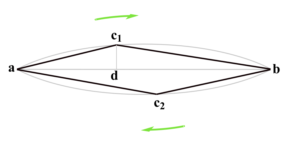Diagram of a plucked string (Image: Amitchell125, CC BY-SA 4.0, via Wikimedia Commons)