Multimedia ComputingUnit 514 min read
Data Compression: Techniques, Algorithms & Applications
Unit 5 of Multimedia Computing explores how data compression reduces file sizes while preserving quality, covering lossless (e.g., Huffman, LZW) and lossy (e.g., JPEG, MP3) methods, their mathematical foundations, and real-world trade-offs in multimedia systems like video streaming and cloud storage.
Why Compression Matters
Data compression is the process of encoding information using fewer bits than the original representation. It is essential for:
- Efficient storage: Saving disk space or cloud storage costs.
- Faster transmission: Reducing bandwidth usage for streaming or downloads.
- Cost savings: Lowering data transfer fees (e.g., mobile internet charges).
Multimedia files (images, audio, video) are highly redundant—they contain repeated patterns, predictable structures, or irrelevant details. Compression exploits these redundancies to shrink file sizes without (or with minimal) quality loss.
Types of Compression
Compression falls into two broad categories, each with distinct trade-offs:
1. Lossless Compression
Definition: Reconstructs the original data exactly after decompression. No information is discarded. Use cases: Text files, spreadsheets, medical images, ZIP archives, PNG images.
How it works:
- Removes redundancy (repeated data) and inefficiency (unnecessary bits).
- Uses entropy coding (e.g., Huffman, Arithmetic) or dictionary-based methods (e.g., LZW).
Example: A text file with repeated words like "the the the" can be compressed by storing "the" once and referencing it later.
2. Lossy Compression
Definition: Sacrifices some data to achieve higher compression ratios. The decompressed data is approximate but visually/audibly similar. Use cases: JPEG images, MP3 audio, MP4 videos, where minor quality loss is acceptable.
How it works:
- Exploits human perception limits (e.g., eyes miss high-frequency details, ears ignore inaudible frequencies).
- Uses quantization (rounding values) or discrete transforms (e.g., DCT in JPEG).
| Feature | Lossless | Lossy |
|---|---|---|
| Quality | Original data preserved | Approximate, may lose details |
| Compression Ratio | Low (2:1 to 4:1) | High (10:1 to 100:1) |
| Use Cases | Text, code, medical data, ZIP | Photos, music, video, MP3, JPEG |
| Reversibility | Fully reversible | Irreversible |
| Example Algorithms | Huffman, LZW, Run-Length Encoding (RLE) | JPEG, MP3, MPEG, AAC |
Key Lossless Compression Techniques
1. Run-Length Encoding (RLE)
How it works:
- Replaces sequences of identical data with a count + value pair.
- Example:
"AAAABBBCCDAA"→(4,A)(3,B)(2,C)(1,D)(2,A)
Limitations:
- Ineffective for files with no repeated patterns (e.g., natural images).
- Works best for binary data (e.g., fax images, simple graphics).
Worked Example:
Compress the string "WWWWWWWWWWWWBBBWWWWWWWWWWWWWW" using RLE.
Solution:
(12,W)(3,B)(15,W)
Real-World Use:
- Fax machines: Transmit black-and-white documents efficiently.
- Simple graphics: Used in early bitmap formats (e.g., BMP RLE).
2. Huffman Coding
How it works:
- Assigns variable-length codes to symbols based on frequency.
- More frequent symbols get shorter codes; rarer symbols get longer codes.
- Uses a binary tree to encode/decode data.
Steps:
- Calculate the frequency of each symbol in the data.
- Build a Huffman tree by merging the two least frequent symbols iteratively.
- Assign codes by traversing the tree (left =
0, right =1).
Example:
Compress the string "ABRACADABRA" using Huffman coding.
| Symbol | Frequency | Huffman Code |
|---|---|---|
| A | 5 | 0 |
| B | 2 | 10 |
| R | 2 | 110 |
| C | 1 | 1110 |
| D | 1 | 1111 |
Encoded string:
"ABRACADABRA" → 0 110 1110 0 110 0 0 0 10 0 110 → 011011100110000100110
Advantages:
- Optimal for symbol frequencies (minimizes expected code length).
- Used in PKZIP, JPEG (for lossless mode), and PNG.
Disadvantage:
- Requires frequency analysis before encoding.
- Not efficient for small files (overhead of storing the tree).
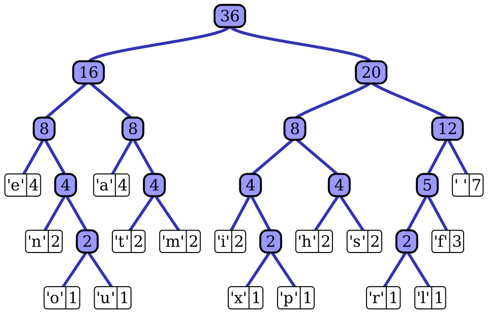 A labelled Huffman tree for the string ABRACADABRA showing symbol frequencies and binary codes. (Image: Meteficha, Public domain, via Wikimedia Commons)
3. Lempel-Ziv-Welch (LZW)
How it works:
- Builds a dynamic dictionary of repeated patterns.
- Replaces repeating sequences with shorter codes.
- Used in GIF, TIFF, and early ZIP formats.
Example:
Compress the string "ABABABABAB" using LZW.
| Step | Input | Dictionary Entry | Output Code |
|---|---|---|---|
| 1 | A | A → 0 | 0 |
| 2 | B | B → 1 | 1 |
| 3 | AB | AB → 2 | 2 |
| 4 | ABAB | (AB)AB → 3 | 3 |
Encoded string: 0 1 2 3
Advantage:
- No need for frequency analysis (adaptive).
- Works well for natural language and images.
Disadvantage:
- Patent issues (original LZW was patented by Unisys).
- Slower than Huffman for some data.
Key Lossy Compression Techniques
1. JPEG (Joint Photographic Experts Group)
How it works:
- Color Space Conversion: RGB → YCbCr (luminance + chrominance).
- Downsampling: Chrominance (color) is subsampled (reduced resolution) because human eyes are less sensitive to color than brightness.
- Discrete Cosine Transform (DCT): Converts image into 8×8 blocks of frequency components.
- Quantization: High-frequency components (less visible) are rounded off.
- Entropy Coding: Huffman or Arithmetic coding compresses the quantized data.
Why it’s effective:
- Exploits psychovisual redundancy (humans don’t notice high-frequency details).
- Achieves 10:1 to 20:1 compression with minimal quality loss.
Worked Example: A 24-bit RGB image (8 bits per channel) is converted to YCbCr. If chrominance is subsampled by 2:1:1, the file size reduces significantly.
Real-World Use:
- Digital cameras: Save photos in JPEG format.
- Web images: Faster loading due to smaller file sizes.
- eSewa/Khalti apps: Profile pictures are often stored as JPEG.
2. MP3 (MPEG-1 Audio Layer III)
How it works:
- Frequency Analysis: Audio is split into 32 frequency bands.
- Psychological Modeling: Removes inaudible frequencies (e.g., below 20Hz or above hearing range).
- Quantization: Reduces precision of less perceptible frequencies.
- Entropy Coding: Huffman coding compresses the data.
Why it’s effective:
- Exploits audio masking (loud sounds hide quieter ones).
- Achieves 10:1 to 12:1 compression with near-CD quality.
Real-World Use:
- Music streaming: Spotify, YouTube Music use MP3/AAC.
- Mobile apps: Pathao’s background music uses compressed audio.
- Radio broadcasts: MP3 is the standard for digital radio.
3. MPEG (Moving Picture Experts Group)
How it works:
- Combines video + audio compression using:
- Temporal Redundancy: Only store changes between frames (motion compensation).
- Spatial Redundancy: Compress each frame like JPEG.
- Entropy Coding: Huffman/Arithmetic coding.
Frame Types:
- I-frame (Intra-coded): Full frame (like JPEG), used as reference.
- P-frame (Predicted): Stores differences from previous I/P frame.
- B-frame (Bidirectional): Stores differences from past and future frames.
Example: A 1-minute 1080p video at 30fps:
- Uncompressed: ~10 GB.
- MPEG-4 (H.264): ~500 MB (20:1 compression).
Real-World Use:
- YouTube/Netflix: Use H.264/H.265 (MPEG variants).
- Video calls: Zoom/Google Meet use VP8/VP9 (MPEG-based).
- Nepali TV: Broadcasts use MPEG-2/DVB standards.
Data Compression in Real-World Systems
1. eSewa & Khalti (Digital Payments)
- Problem: Transaction data (e.g., QR codes, payment logs) must be fast and small.
- Solution:
- Lossless compression (e.g., Zlib) for transaction records.
- Base64 encoding (not compression, but reduces storage for text data).
- Impact: Faster processing, lower bandwidth usage.
2. Daraz/Nepali Online Shopping
- Problem: Product images/videos must load quickly on slow networks.
- Solution:
- JPEG/WebP for photos (lossy compression).
- MP4/H.265 for product videos (high compression).
- Impact: Faster page loads, better user experience.
3. Ncell/NTC (Mobile Data)
- Problem: High data usage for streaming/video calls.
- Solution:
- Adaptive Bitrate Streaming (ABR): Adjusts video quality (e.g., 720p → 480p) based on network.
- HTTP/3 + QUIC: Reduces latency and improves compression efficiency.
- Impact: Lower data costs for users.
4. NEPSE (Stock Market Data)
- Problem: Real-time stock prices generate huge data volumes.
- Solution:
- Delta encoding: Store only changes in prices (not full values).
- Columnar storage: Compress numerical data efficiently (e.g., Parquet format).
- Impact: Faster analytics, lower storage costs.
5. Kathmandu Traffic Management (Simulated)
Scenario: Traffic cameras generate 1000s of images/hour. Compressing them reduces storage and transmission costs. Solution:
- JPEG for still images (80% quality → 70% size reduction).
- H.265 for video feeds (4K → 1080p with minimal quality loss). Impact: Easier AI processing for traffic monitoring.
Mathematical Foundations
1. Entropy and Information Theory
- Entropy (H): Measures uncertainty in data.
- Example: A fair coin flip has bit (maximum entropy).
- Compression goal: Reduce entropy by removing redundancy.
2. Rate-Distortion Theory
- Trade-off: Higher compression → More distortion.
- Example: MP3 at 128 kbps vs. 320 kbps (same audio, different quality).
3. Quantization
- Process: Mapping input values to a smaller set (e.g., 256 colors → 16 colors).
- Example: In JPEG, DCT coefficients are quantized to reduce precision.
Comparison of Compression Standards
| Standard | Type | Use Case | Compression Ratio | Quality Loss |
|---|---|---|---|---|
| ZIP | Lossless | Documents, backups | 2:1 to 4:1 | None |
| JPEG | Lossy | Photos, web images | 10:1 to 20:1 | Moderate |
| MP3 | Lossy | Music, podcasts | 10:1 to 12:1 | Low |
| H.264 | Lossy | Videos, streaming | 20:1 to 50:1 | Low-Moderate |
| PNG | Lossless | Graphics, screenshots | 2:1 to 5:1 | None |
| GIF | Lossless* | Simple animations | 3:1 to 10:1 | None (256 colors) |
| FLAC | Lossless | High-fidelity audio | 2:1 to 3:1 | None |
*GIF uses LZW (lossless for pixel data but limited to 256 colors).
Exam Tip
Define clearly:
- Lossless vs. lossy (give examples).
- Entropy, quantization, and DCT (for JPEG/MP3).
Algorithmic steps:
- Explain Huffman coding or LZW with a small example.
- Describe JPEG/MPEG pipelines in 3-4 steps.
Real-world applications:
- Link compression to eSewa (data efficiency), YouTube (video streaming), or Ncell (bandwidth savings).
- Compare PNG vs. JPEG for different use cases.
Maths:
- Calculate entropy for a given symbol set.
- Explain rate-distortion trade-off with an example (e.g., MP3 bitrate vs. quality).
Diagrams:
- Draw a Huffman tree or MPEG frame types in the exam if asked for a visual explanation.
Common mistakes to avoid:
- Confusing RLE with Huffman (RLE is for runs, Huffman is for frequencies).
- Forgetting that JPEG is lossy while PNG is lossless.
- Not explaining why a method works (e.g., "because humans can’t see high frequencies").
Mermaid Diagram: Compression Techniques Classification
Based on the TU BIT syllabus for Multimedia Computing (BIT356), unit 5.
Discussion
Loading…