Data Warehousing and Data MiningUnit 67 min read
Classification & Prediction: Models, Trees, Rules & Evaluation
Unit 6 of Data Warehousing and Data Mining covers supervised learning techniques—decision trees, rule-based classifiers, Bayesian networks, neural networks, and evaluation metrics (accuracy, precision, recall)—with real-world applications in fraud detection, customer segmentation, and predictive maintenance.
Key Concepts and Techniques
1. Classification vs. Prediction
Classification and prediction are both supervised learning tasks, but they differ in their output types:
- Classification: Predicts discrete class labels (e.g., spam/not spam, loan approved/rejected).
- Prediction: Predicts continuous numerical values (e.g., house price, stock price).
classDiagram
    class SupervisedLearning {
        +Input: Labeled Data
        +Output: Predicted Labels/Values
    }
    class Classification {
        +Output: Discrete Classes
        +Examples: Decision Trees, Naive Bayes
    }
    class Prediction {
        +Output: Continuous Values
        +Examples: Linear Regression, Neural Networks
    }
    SupervisedLearning <|-- Classification
    SupervisedLearning <|-- Prediction
2. Decision Trees
Decision trees are hierarchical models that split data based on feature values to classify instances.
How Decision Trees Work
- Root Node: Represents the entire dataset.
- Internal Nodes: Represent features (e.g., age, income).
- Leaf Nodes: Represent class labels (e.g., "Buy" or "Not Buy").
Splitting Criteria:
- Gini Index: Measures impurity (lower = better split).
- Entropy: Measures disorder (lower = better split).
- Information Gain: Difference in entropy before/after split.
Worked Example: Customer Purchase Prediction
Suppose we have a dataset of customers with features:
- Age: ≤30, >30
- Income: ≤50k, >50k
- Class: Buy (Yes/No)
Step 1: Calculate Entropy of the Root Node Total customers = 14
- Buy (Yes) = 9
- Buy (No) = 5 Entropy =
Step 2: Split on "Income" (Best Feature)
- Income ≤50k: 7 customers (Buy=3, No=4)
- Income >50k: 7 customers (Buy=6, No=1) Entropy after split:
- Left:
- Right: Weighted entropy = Information Gain = 0.94 - 0.79 = 0.15 (Best split!)
Step 3: Build the Tree
            [Income]
          /           \
   ≤50k             >50k
 /    \           /     \
Buy?   No      Buy      No
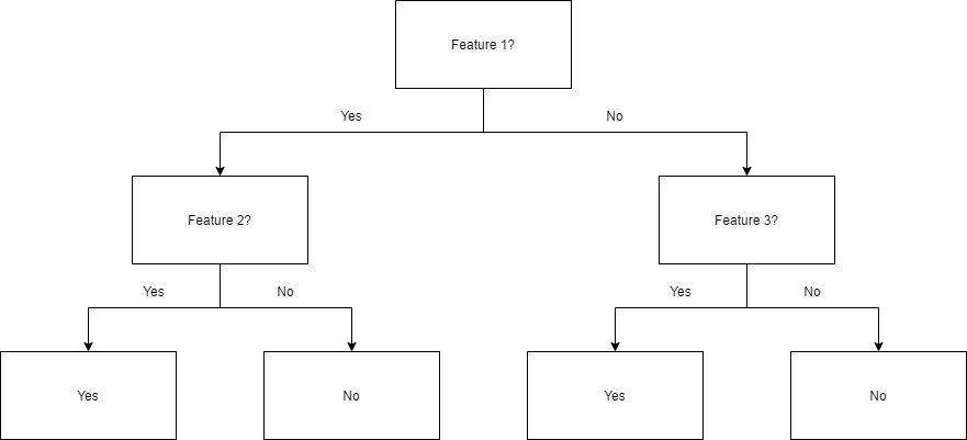 A simple decision tree for customer purchase prediction (Image: CollaborativeGeneticist, CC BY-SA 4.0, via Wikimedia Commons)
3. Rule-Based Classifiers
Rule-based classifiers (e.g., Association Rules, If-Then Rules) are derived from frequent patterns.
Example: Market Basket Analysis (Daraz/Khalti)
Suppose we mine transaction data to find:
- Rule: {Diapers} → {Beer} (Support=10%, Confidence=70%)
- Support: % of transactions containing both items.
- Confidence: % of transactions with Diapers that also have Beer.
Worked Example: Khalti Transaction Data
| Transaction ID | Items Purchased |
|---|---|
| T1 | Diapers, Beer, Bread |
| T2 | Diapers, Beer |
| T3 | Bread, Milk |
Rule: {Diapers} → {Beer}
- Support = (2/3) × 100% ≈ 66.67%
- Confidence = (2/2) × 100% = 100%
4. Bayesian Networks
Bayesian networks use probability to model dependencies between variables.
Example: Loan Approval Prediction (Nepal Bank)
Suppose a bank uses:
- Features: Income, Credit Score, Employment Status
- Target: Loan Approved (Yes/No)
Conditional Probability Table (CPT) Example:
| Income | Credit Score | Employment | Loan Approved |
|---|---|---|---|
| High | Good | Yes | 0.9 |
| Low | Poor | No | 0.1 |
Worked Example: Probability Calculation
- P(Loan=Yes | Income=High, Credit=Good, Employed=Yes) = 0.9
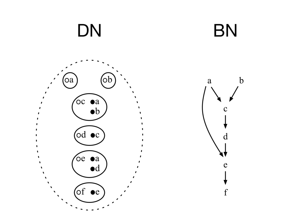 Loan approval Bayesian network (Image: Andre.eds, CC BY-SA 4.0, via Wikimedia Commons)
5. Neural Networks for Classification
Neural networks use layers of nodes to learn complex patterns.
Structure of a Neural Network
Input Layer → Hidden Layers → Output Layer
- Activation Functions: Sigmoid, ReLU, Softmax.
- Loss Functions: Cross-Entropy (Classification), MSE (Regression).
Worked Example: Spam Detection (eSewa Messages)
- Input: Word embeddings (e.g., "free offer" = [0.8, -0.2, ...])
- Hidden Layer: Weights adjust to detect spam patterns.
- Output: Probability of spam (0 to 1).
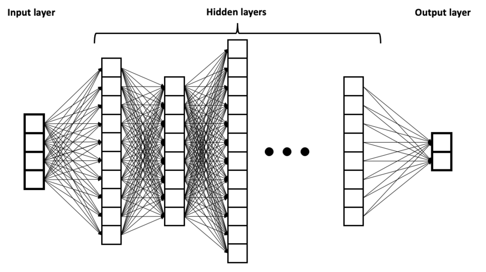 A 3-layer neural network for spam detection (Image: BrunelloN, CC BY-SA 4.0, via Wikimedia Commons)
6. Evaluation Metrics
| Metric | Formula | When to Use |
|---|---|---|
| Accuracy | (TP + TN) / (TP + TN + FP + FN) | Balanced datasets |
| Precision | TP / (TP + FP) | Minimize false positives |
| Recall | TP / (TP + FN) | Minimize false negatives |
| F1-Score | 2 × (Precision × Recall) / (P+R) | Imbalanced datasets |
Worked Example: Fraud Detection (Ncell)
- TP (True Positive): Fraud detected correctly.
- FP (False Positive): Legitimate transaction flagged as fraud.
- Precision: If 90% of flagged transactions are fraud, precision = 0.9.
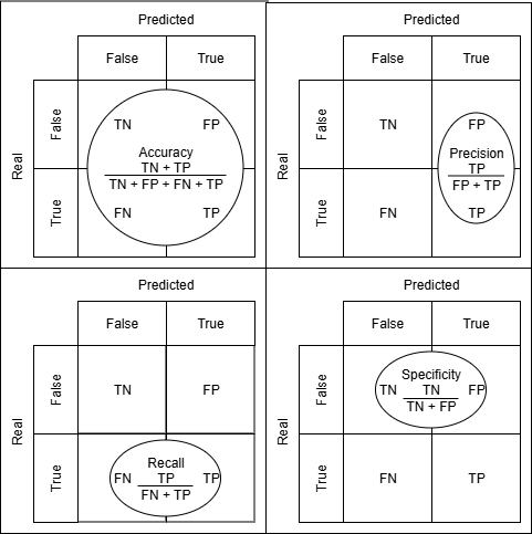 Confusion matrix for fraud detection (Image: Hssiqueira, CC0, via Wikimedia Commons)
In the Real World
- Khalti/E-Sewa: Uses decision trees to detect fraudulent transactions by analyzing spending patterns, device location, and transaction history.
- Daraz: Applies association rule mining to recommend products (e.g., "Customers who bought X also bought Y").
- Nepal Rastra Bank (NRB): Employs Bayesian networks to assess loan risks by combining economic indicators (inflation, GDP growth) with borrower data.
Exam Tip
- Decision Trees: Always calculate information gain or Gini index for splits.
- Rule Mining: Remember support, confidence, and lift for association rules.
- Evaluation Metrics: Know when to use precision vs. recall (e.g., medical tests vs. spam filters).
- Neural Networks: Understand activation functions (ReLU vs. Sigmoid) and loss functions (Cross-Entropy for classification).
Summary Table of Classifiers
| Method | Strengths | Weaknesses |
|---|---|---|
| Decision Trees | Easy to interpret, fast training | Prone to overfitting |
| Rule-Based | Human-readable rules | Scalability issues |
| Bayesian Networks | Handles uncertainty well | Requires expert knowledge |
| Neural Networks | High accuracy for complex data | Black-box, needs large data |
Based on the TU BIT syllabus for Data Warehousing and Data Mining, unit 6.
Discussion
Loading…