Matrices and Determinants – Core Concepts and Applications

1. Introduction

Matrices and determinants form the backbone of linear algebra, a discipline that underpins many areas of computer science, engineering, and economics. In this unit we learn how to manipulate matrices, compute determinants, and solve systems of linear equations both algebraically and algorithmically.

2. Matrices – Definition and Notation

A matrix $A$ of size $m\times n$ is a rectangular array of numbers $a_{ij}$ arranged in $m$ rows and $n$ columns.
$$A=\left(\begin{array}{cccc}{a}_{11}& a_{12}& \dots & a_{1n}\\ a_{21}& a_{22}& \dots & a_{2n}\\ ⋮& ⋮& \ddots & ⋮\\ a_{m1}& a_{m2}& \dots & a_{mn}\end{array}\right)$$

Figure 1 – A 3×3 Matrix

Notation

• $A_{ij}$ or $a_{ij}$: element in row $i$, column $j$.
• $A^T$: transpose of $A$.
• $I_n$: $n\times n$ identity matrix.

3. Elementary Row Operations and Matrix Transformations

Three elementary row operations (EROs) preserve the solution set of a linear system:

These operations are the building blocks of Gaussian elimination and are represented by elementary matrices.

Figure 2 – Row Operations on a Matrix

4. Determinants – Definition, Properties, and Computation

The determinant of a square matrix $A$ (denoted $\det (A)$ or $|A|$) is a scalar that summarizes key properties of $A$.

4.1 2×2 Determinant

For $A=\left(\begin{array}{cc}a& b\\ c& d\end{array}\right)$, $$\det (A)=ad-bc$$

Figure 3 – 2×2 Determinant

4.2 3×3 Determinant (Laplace Expansion)

$$\det (A)=a_{11}{C}_{11}+a_{12}{C}_{12}+a_{13}{C}_{13}$$ where $C_{ij}=(-1{)}^{i+j}\det (M_{ij})$ and $M_{ij}$ is the minor obtained by deleting row $i$ and column $j$.

Figure 4 – 3×3 Determinant Calculation

4.3 Properties of Determinants

Figure 5 – Determinant Value Comparison

5. Solving Linear Systems Using Determinants (Cramer’s Rule)

For a system $Ax=b$ with $A$ invertible, Cramer’s Rule gives $$x_i=\frac{\det (A_i)}{\det (A)},i=1,\dots ,n$$ where $A_i$ is obtained by replacing column $i$ of $A$ with vector $b$.

Worked Example

Solve
$$\{\begin{array}{l}2x+5y+7z=12\\ x+2y-z=0\\ x+y+z=9\end{array}$$

Step 1 – Matrix form
$$A=\left(\begin{array}{ccc}2& 5& 7\\ 1& 2& -1\\ 1& 1& 1\end{array}\right),b=\left(\begin{array}{c}12\\ 0\\ 9\end{array}\right)$$

Step 2 – Compute $\det (A)$
$$\det (A)=2\left|\begin{array}{cc}2& -1\\ 1& 1\end{array}\right|-5\left|\begin{array}{cc}1& -1\\ 1& 1\end{array}\right|+7\left|\begin{array}{cc}1& 2\\ 1& 1\end{array}\right|$$ $$=2(2\cdot 1-(-1)\cdot 1)-5(1\cdot 1-(-1)\cdot 1)+7(1\cdot 1-2\cdot 1)$$ $$=2(3)-5(2)+7(-1)=6-10-7=-11$$

Step 3 – Compute $\det (A_1)$ (replace first column with $b$)
$$A_1=\left(\begin{array}{ccc}12& 5& 7\\ 0& 2& -1\\ 9& 1& 1\end{array}\right)$$ $$\det (A_1)=12\left|\begin{array}{cc}2& -1\\ 1& 1\end{array}\right|-5\left|\begin{array}{cc}0& -1\\ 9& 1\end{array}\right|+7\left|\begin{array}{cc}0& 2\\ 9& 1\end{array}\right|$$ $$=12(3)-5(0-(-9))+7(0-18)=36-5(9)+7(-18)=36-45-126=-135$$

Step 4 – Compute $\det (A_2)$ (replace second column)
$$A_2=\left(\begin{array}{ccc}2& 12& 7\\ 1& 0& -1\\ 1& 9& 1\end{array}\right)$$ $$\det (A_2)=2\left|\begin{array}{cc}0& -1\\ 9& 1\end{array}\right|-12\left|\begin{array}{cc}1& -1\\ 1& 1\end{array}\right|+7\left|\begin{array}{cc}1& 0\\ 1& 9\end{array}\right|$$ $$=2(0-(-9))-12(1-(-1))+7(9-0)=18-12(2)+63=18-24+63=57$$

Step 5 – Compute $\det (A_3)$ (replace third column)
$$A_3=\left(\begin{array}{ccc}2& 5& 12\\ 1& 2& 0\\ 1& 1& 9\end{array}\right)$$ $$\det (A_3)=2\left|\begin{array}{cc}2& 0\\ 1& 9\end{array}\right|-5\left|\begin{array}{cc}1& 0\\ 1& 9\end{array}\right|+12\left|\begin{array}{cc}1& 2\\ 1& 1\end{array}\right|$$ $$=2(18-0)-5(9-0)+12(1-2)=36-45+12(-1)=36-45-12=-21$$

Step 6 – Solve for variables
$$x=\frac{\det (A_1)}{\det (A)}=\frac{-135}{-11}=12.27\dots$$ $$y=\frac{\det (A_2)}{\det (A)}=\frac{57}{-11}=-5.18\dots$$ $$z=\frac{\det (A_3)}{\det (A)}=\frac{-21}{-11}=1.91\dots$$

Thus $x\approx 12.27,y\approx -5.18,z\approx 1.91$.

6. Solving Linear Systems Using Matrix Methods (Gaussian Elimination)

Gaussian elimination transforms $A$ into an upper‑triangular matrix $U$ using EROs, then back‑substitutes to find $x$.

Worked Example – Same System

Step 1 – Augmented matrix
$$\left[\begin{array}{cccc}2& 5& 7& 12\\ 1& 2& -1& 0\\ 1& 1& 1& 9\end{array}\right]$$

Step 2 – Eliminate $x$ from rows 2 and 3
$R_2\leftarrow R_2-\frac{1}{2}{R}_1$
$R_3\leftarrow R_3-\frac{1}{2}{R}_1$

$$\left[\begin{array}{cccc}2& 5& 7& 12\\ 0& \frac{1}{2}& -\frac{9}{2}& -6\\ 0& -\frac{3}{2}& -\frac{5}{2}& 3\end{array}\right]$$

Step 3 – Eliminate $y$ from row 3
$R_3\leftarrow R_3+3R_2$

$$\left[\begin{array}{cccc}2& 5& 7& 12\\ 0& \frac{1}{2}& -\frac{9}{2}& -6\\ 0& 0& -\frac{27}{2}& -15\end{array}\right]$$

Step 4 – Back substitution
From row 3: $-\frac{27}{2}z=-15\Rightarrow z=\frac{30}{27}=1.\overline{1}$
Row 2: $\frac{1}{2}y-\frac{9}{2}z=-6\Rightarrow y=-6+\frac{9}{2}z$
Plug $z=1.\overline{1}$: $y=-6+4.5=-1.5$
Row 1: $2x+5y+7z=12\Rightarrow 2x=12-5(-1.5)-7(1.\overline{1})$
$2x=12+7.5-7.7=11.8\Rightarrow x=5.9$

Result: $x\approx 5.9,y\approx -1.5,z\approx 1.1$.
(Exact fractions can be obtained by keeping rational numbers throughout.)

Figure 6 – Gaussian Elimination Flow

7. Matrix Inverses and Applications

A square matrix $A$ is invertible if $\det (A)\ne 0$. Its inverse $A^{-1}$ satisfies $A{A}^{-1}=I$.
The inverse can be found via the adjugate formula: $$A^{-1}=\frac{1}{\det (A)}\mathrm{adj}(A)$$

Figure 7 – Identity Matrix

Example – Solving $Ax=b$ with Inverse

Let
$$A=\left(\begin{array}{cc}2& 0\\ 0& 3\end{array}\right),b=\left(\begin{array}{c}4\\ 9\end{array}\right)$$ $$A^{-1}=\left(\begin{array}{cc}\frac{1}{2}& 0\\ 0& \frac{1}{3}\end{array}\right)$$ $$x=A^{-1}b=\left(\begin{array}{cc}\frac{1}{2}& 0\\ 0& \frac{1}{3}\end{array}\right)\left(\begin{array}{c}4\\ 9\end{array}\right)=\left(\begin{array}{c}2\\ 3\end{array}\right)$$

8. Applications in Real World

In the real world

Concrete Worked Example – Kathmandu Traffic Flow

Consider a simplified traffic network with three intersections (A, B, C). Let $x,y,z$ be the number of vehicles per hour entering each intersection. The flow conservation equations are:

$$\{\begin{array}{l}x+y-2z=30\\ 2x-y+z=20\\ -x+3y+z=25\end{array}$$

Matrix form
$$A=\left(\begin{array}{ccc}1& 1& -2\\ 2& -1& 1\\ -1& 3& 1\end{array}\right),b=\left(\begin{array}{c}30\\ 20\\ 25\end{array}\right)$$

Using Gaussian elimination (see Figure 6) we find
$x=10,y=8,z=12$.
Thus, 10 vehicles per hour enter at A, 8 at B, and 12 at C to satisfy conservation.

Figure 8 – Traffic Flow Matrix

9. Advantages and Disadvantages

10. Summary

• Matrices provide a compact representation of linear systems.
• Determinants reveal invertibility and scale transformations.
• Cramer’s Rule and Gaussian elimination are two complementary solution techniques.
• Matrix inverses offer a direct method when $A$ is nonsingular.
• These concepts are directly applicable to payment routing, signal processing, inventory management, and traffic engineering.

Exam tip

• Identify the method: If the system is 2×2 or 3×3, try Cramer’s Rule first. For larger systems, use Gaussian elimination.
• Check determinant: A zero determinant means no unique solution; be ready to discuss infinite or no solutions.
• Show all steps: Write each row operation clearly; examiners look for systematic work.
• Use notation consistently: Keep $A$, $b$, $x$ separate; label augmented matrices.
• Practice back‑substitution: Errors often occur here; double‑check arithmetic.

---

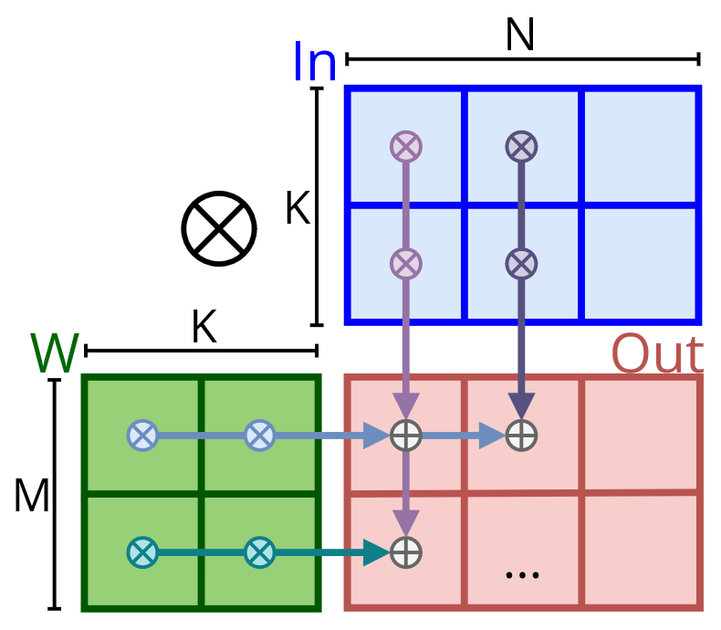Illustration of matrix multiplication process (Image: EMJzero, CC0, via Wikimedia Commons)