Measures of Dispersion: Range, Quartiles, SD, Variance & Real-World Spread

TAKEAWAYS:

• Range shows total spread but ignores internal distribution (e.g., Daraz order delays).
• Quartile deviation measures middle 50% spread (used in Pokhara household expenditure analysis).
• Variance and standard deviation quantify average deviation from the mean (critical for Ncell call-drop probability).
• Coefficient of variation compares dispersion across different scales (e.g., NEPSE stock volatility).
• Real-world ties: Bank loan interest (SD), Pathao driver earnings (quartiles), Kathmandu traffic routes (range).
• Exam focus: Formula derivation, interpretation, and confidence interval calculations (e.g., "95% confidence limits for population mean").

---

1. Why Dispersion Matters: Beyond the Average

Statistics often report a mean (e.g., average salary = Rs 40,000), but this hides how spread out the data is. Dispersion measures answer:

• "Are most salaries close to Rs 40,000, or do some earn Rs 10,000 while others earn Rs 100,000?"
• "Is this dataset reliable for predictions?"

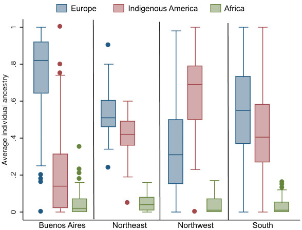A box plot showing median, quartiles, and outliers for a dataset. (Image: Sergio Avena, Marc Via, Elad Ziv, Eliseo J. Pérez-Stable, Ch, CC BY 2.5, via Wikimedia Commons)

Key Definitions

---

2. Range: The Simplest (But Crude) Measure

How it works:

• Identify the minimum and maximum values in your dataset.
• Subtract: $R=X_{\text{max}}-X_{\text{min}}$.

Example 1: Daraz Order Delivery Times (in hours) Data: 24, 36, 48, 60, 72, 84, 96, 120, 144, 168

• Range = 168 – 24 = 144 hours (4 days!).
• Problem: One delayed order skews the range. A better measure? → Quartiles.

Real-World Tie:

• NTC Internet Speeds: Range alone can’t tell if most users get 50 Mbps or if speeds vary wildly. Quartiles or SD are better.

---

3. Quartile Deviation: Ignoring Outliers

Why? Range is sensitive to extremes. Quartile deviation focuses on the middle 50% of data.

Steps to Calculate Q1, Q2 (Median), Q3

1. Order data: $X_1,X_2,...,X_n$.
2. Find Q2 (Median):
   • If $n$ is odd: middle value.
   • If even: average of two middle values.
3. Find Q1 (1st Quartile): Median of the lower half (excluding Q2 if $n$ is odd).
4. Find Q3 (3rd Quartile): Median of the upper half.

Example 2: Pokhara Household Expenditure (Rs ’00)

Step-by-Step:

1. Cumulative frequencies:

   • 30–50: 54
   • 50–70: 54 + 100 = 154
   • 70–90: 154 + 140 = 294
   • 90–110: 294 + 300 = 594 (Q2 lies here)
   • 110–130: 594 + 230 = 824
   • 130–150: 824 + 176 = 1000

2. Q2 (Median):

   • $\frac{1000}{2}=500$th value falls in 90–110.
   • $Q2=90+\left(\frac{500-294}{300}\times 20\right)=90+17.2=107.2$.

3. Q1 (25th percentile):

   • $\frac{1000}{4}=250$th value falls in 70–90.
   • $Q1=70+\left(\frac{250-154}{140}\times 20\right)=70+13.57=83.57$.

4. Q3 (75th percentile):

   • $\frac{3\times 1000}{4}=750$th value falls in 110–130.
   • $Q3=110+\left(\frac{750-594}{230}\times 20\right)=110+15.65=125.65$.

5. Quartile Deviation (QD):

   • $QD=\frac{Q3-Q1}{2}=\frac{125.65-83.57}{2}=21.04$.

Interpretation:

• The middle 50% of households spend between Rs 83.57k and Rs 125.65k.
• Coefficient of Quartile Deviation: $\text{CQD}=\frac{QD}{Q2}\times 100=\frac{21.04}{107.2}\times 100\approx 19.63\%$.

---

4. Variance and Standard Deviation: The Gold Standard

Why? They measure average deviation from the mean, accounting for all data points.

Formulas

Example 3: Ncell Call Drop Probability A sample of 5 calls has drop times (seconds): 2, 4, 4, 5, 7.

1. Mean ($\bar{X}$): $\frac{2+4+4+5+7}{5}=4.4$ sec.
2. Variance ($s^2$): $$\begin{array}{rl}{s}^2& =\frac{(2-4.4{)}^2+(4-4.4{)}^2+(4-4.4{)}^2+(5-4.4{)}^2+(7-4.4{)}^2}{5-1}\\ & =\frac{5.76+0.16+0.16+0.36+6.76}{4}\\ & =\frac{13.2}{4}=3.3{\text{ sec}}^2.\end{array}$$
3. Standard Deviation ($s$): $\sqrt{3.3}\approx 1.82$ sec.

Interpretation:

• Calls drop on average 1.82 seconds from the mean drop time of 4.4 sec.
• High SD → Inconsistent service (some calls drop instantly, others last longer).

---

5. Coefficient of Variation (CV): Comparing Apples to Oranges

Problem: SD alone can’t compare dispersion across datasets with different units (e.g., Rs vs. hours). Solution: CV standardizes SD as a percentage of the mean.

Formula: $$CV=\frac{\sigma }{\mu }\times 100$$

Example 4: NEPSE vs. Daraz Sales Volatility

Insight:

• NEPSE stocks are slightly more volatile (16% vs. 15%) despite higher absolute SD.
• Use CV when comparing risk across industries (e.g., bank loans vs. stock investments).

---

6. Real-World Applications

A. Bank Loan Interest Rates (Standard Deviation)

Scenario: A bank offers loans with an average interest rate of 10% but varies by customer.

• Low SD (e.g., 1%): Most customers pay 9–11% → Predictable revenue.
• High SD (e.g., 5%): Some pay 5%, others 15% → Higher risk for the bank.

Example 5: Kathmandu Bank Loan Data

Calculations:

1. Mean ($\mu$): 11% (weighted average).
2. Variance (${\sigma }^2$):
   • Convert to midpoints: 9, 11, 13, 15.
   • ${\sigma }^2=\frac{(9-11{)}^2\times 100+(11-11{)}^2\times 200+(13-11{)}^2\times 150+(15-11{)}^2\times 50}{500}$.
   • ${\sigma }^2=\frac{400+0+450+800}{500}=3.1$.
3. SD ($\sigma$): $\sqrt{3.1}\approx 1.76\%$.

Bank’s Decision:

• Low SD (1.76%) → Stable revenue; can plan budgets confidently.
• If SD were 5%, the bank might offer risk buffers or higher default protections.

B. Pathao Driver Earnings (Quartiles)

Scenario: Pathao drivers earn Rs 30,000–50,000/month, but some earn as low as Rs 10,000.

• Range: Rs 40,000 (misleading if outliers exist).
• Quartiles:
  • Q1 (25th percentile): Rs 20,000
  • Q3 (75th percentile): Rs 40,000
  • Interquartile Range (IQR): Rs 20,000 → Shows middle 50% earn Rs 20k–40k.

Why Quartiles?

• Ignores top 25% (high earners) and bottom 25% (struggling drivers).
• Helps Pathao target support to drivers in Q1 (e.g., training programs).

C. Kathmandu Traffic Congestion (Range vs. SD)

Scenario: Traffic police measure vehicle speeds (km/h) on Ring Road.

• Range: 20–80 km/h → 60 km/h spread (seems bad).
• SD: 10 km/h → Most cars travel within 10 km/h of the mean (50 km/h).
• Insight: Range overstates congestion; SD shows most traffic is slow but stable.

---

7. Comparing Dispersion Measures

---

8. Common Pitfalls

1. Using Range for skewed data: A single outlier (e.g., a Rs 1M salary in a Rs 50k dataset) can distort it.
2. Ignoring sample vs. population formulas:
   • Population: Divide by $N$.
   • Sample: Divide by $n-1$ (Bessel’s correction).
3. Misinterpreting SD:
   • SD = 0 → All values are identical.
   • High SD → Data is widely spread (e.g., stock prices).
4. CV for zero mean: Undefined (e.g., temperature changes around 0°C).

---

9. Worked Example: Past Exam Question

Question: A sample of 500 bulbs has an average life of 1400 hours with a standard deviation of 30 hours. Find the 95% confidence limits for the population mean.

Solution:

1. Given:

   • Sample mean ($\bar{X}$) = 1400 hours.
   • Sample SD ($s$) = 30 hours.
   • Sample size ($n$) = 500.
   • Confidence level = 95% → $z=1.96$ (from Z-table).

2. Standard Error (SE): $$SE=\frac{s}{\sqrt{n}}=\frac{30}{\sqrt{500}}\approx 1.34$$

3. Confidence Interval: $$\text{Margin of Error}=z\times SE=1.96\times 1.34\approx 2.63$$ $$\text{CI}=\bar{X}\pm \text{ME}=1400\pm 2.63\to [1397.37,1402.63]\text{ hours}.$$

Interpretation:

• We are 95% confident the true population mean bulb life is between 1397 and 1403 hours.

---

10. Exam Tip: How to Score Full Marks

1. Show all steps: Examiners deduct marks for skipped calculations.
   • Example: For variance, write: $${\sigma }^2=\frac{\sum X_i^2}{N}-{\mu }^2$$
2. Label units: Always specify units (e.g., "Rs ’00", "seconds", "km/h").
3. Interpret results:
   • Bad: "SD = 10".
   • Good: "The standard deviation of 10 hours means most calls drop within ±10 seconds of the average drop time."
4. Use real-world context:
   • For quartiles: "This shows 50% of households spend between Rs X and Rs Y."
5. Common exam traps:
   • Forget Bessel’s correction ($n-1$) for sample variance.
   • Mix up population/sample formulas.
   • Ignore cumulative frequencies in grouped data (e.g., quartile calculation).

Mermaid Diagram: Exam Checklist

---

In the Real World

1. eSewa Transaction Delays:

   • Measure: Standard deviation of processing times.
   • Why? Low SD means consistent service; high SD means some users wait much longer.
   • Example: If SD = 5 seconds, most transactions take ~mean ±5 sec. If SD = 20 sec, some users face delays.

2. Khalti Loan Approvals:

   • Measure: Coefficient of variation of loan amounts.
   • Why? Compares risk across different loan sizes (e.g., Rs 50k vs. Rs 500k loans).
   • Example: If CV = 20% for Rs 50k loans but 50% for Rs 500k loans, the bank may require stricter checks for larger loans.

3. Daraz Order Fulfillment:

   • Measure: Quartile deviation of delivery times.
   • Why? Ignores the fastest/slowest 25% of orders to focus on typical performance.
   • Example: If Q1 = 2 days and Q3 = 5 days, Daraz knows half its orders take 2–5 days to deliver.

4. NTC Internet Speed Ads:

   • Measure: Range vs. standard deviation.
   • Why? Ads might claim "up to 100 Mbps" (range), but SD shows if most users get 50 Mbps or speeds vary wildly.

5. NEPSE Stock Volatility:

   • Measure: Coefficient of variation of daily returns.
   • Why? Investors compare CV across stocks to pick less risky options.
   • Example: Stock A (mean return 5%, SD 2%) has CV = 40%; Stock B (mean 10%, SD 8%) has CV = 80%. Stock A is less volatile per unit of return.

6. Ncell Network Coverage:

   • Measure: Standard deviation of signal strength (dBm).
   • Why? Low SD means consistent coverage; high SD means some areas have weak signals.
   • Example: If SD = 5 dBm, most users experience signal within ±5 dBm of the mean.