Artificial IntelligenceUnit 88 min read

Neural Networks – Foundations, Training, and Applications

Unit 8 of Artificial Intelligence: introduces neural network concepts, architectures, training algorithms, and real‑world applications.

Padhai · Based on the official syllabus and past papers
Updated 3 Oct 2026

Key points

Neural networks model complex functions using layers of weighted neurons and activation functions.
Training relies on gradient descent and back‑propagation to minimise loss functions.
Regularisation techniques (dropout, L1/L2, early stopping) combat over‑fitting.
Convolutional, recurrent, auto‑encoder and GAN architectures extend basic feed‑forward nets for vision, sequence and generative tasks.
Neural nets power everyday services such as fraud detection in e‑wallets, image search in Google, and voice assistants in smartphones.

Introduction

Artificial Neural Networks (ANNs) are computational models inspired by the biological brain. A neuron receives inputs $x_{i}$ , multiplies them by weights $w_{i}$ , adds a bias $b$ , and applies a non‑linear activation function $ϕ$ to produce an output $y$ :

A network is a directed acyclic graph of such neurons organized in layers. The simplest form, a feed‑forward neural network (FNN), propagates information from input to output without cycles.

Basic Building Blocks

Neuron and Activation Functions

Function	Formula	Domain	Typical Use
Linear	$f (x) = x$	$R$	Output layer for regression
Sigmoid	$σ (x) = \frac{1}{1 + e ^{- x}}$	$R$	Binary classification, hidden layers (historical)
Tanh	$tanh (x) = \frac{e ^{x} - e ^{- x}}{e ^{x} + e ^{- x}}$	$R$	Hidden layers (zero‑centered)
ReLU	$ReLU (x) = max (0, x)$	$R$	Hidden layers (efficient)
Leaky ReLU	$α x$ if $x < 0$ else $x$	$R$	Mitigates dying ReLU
Softmax	$softmax (z_{i}) = \frac{e ^{z_{i}}}{\sum _{j} e ^{z_{j}}}$	$R^{k}$	Multi‑class output

Common activation functions: Sigmoid (saturates at extremes), ReLU (linear for x > 0), Linear (no transformation).

Loss Functions

Task	Loss	Formula
Regression	Mean Squared Error (MSE)	$\frac{1}{m} \sum_{i = 1}^{m} (y_{i} - \overset{y}{^}_{i})^{2}$
Binary Classification	Binary Cross‑Entropy	$- \frac{1}{m} \sum_{i = 1}^{m} [y_{i} lo g \overset{y}{^}_{i} + (1 - y_{i}) lo g (1 - \overset{y}{^}_{i})]$
Multi‑class	Categorical Cross‑Entropy	$- \frac{1}{m} \sum_{i = 1}^{m} \sum_{k = 1}^{K} y_{ik} lo g \overset{y}{^}_{ik}$

Training a Neural Network

Gradient Descent

Weights are updated iteratively:

Gradient descent steps: moving from initial θ toward the loss minimum.

where $η$ is the learning rate and $L$ the loss.

Back‑Propagation

The chain rule propagates gradients from output to input layers. For a single hidden neuron $h$ with output $a_{h} = ϕ (z_{h})$ and output neuron $o$ with $a_{o} = ϕ (z_{o})$ :

Compute error at output: $δ_{o} = (a_{o} - y) ϕ^{'} (z_{o})$ .
Propagate to hidden: $δ_{h} = w_{h o} δ_{o} ϕ^{'} (z_{h})$ .
Update weights:
$w_{h o} \leftarrow w_{h o} - η a_{h} δ_{o}, w_{ih} \leftarrow w_{ih} - η x_{i} δ_{h}$

Worked Example

Consider a network with one input $x = 0.5$ , one hidden neuron, one output neuron.
Weights: $w_{ih} = 0.4$ , $b_{h} = 0.1$ ; $w_{h o} = 0.3$ , $b_{o} = 0.2$ .
Activation: ReLU. Target $y = 1$ .

Forward pass:
$z_{h} = 0.4 \times 0.5 + 0.1 = 0.3$ → $a_{h} = ReLU (0.3) = 0.3$ .
$z_{o} = 0.3 \times 0.3 + 0.2 = 0.29$ → $a_{o} = ReLU (0.29) = 0.29$ .
Loss (MSE): $L = \frac{1}{2} (1 - 0.29)^{2} = 0.245$ .
Gradients:
$δ_{o} = (0.29 - 1) \times 1 = - 0.71$ .
$δ_{h} = 0.3 \times (- 0.71) \times 1 = - 0.213$ .
Weight updates ( $η = 0.1$ ):
$w_{h o} \leftarrow 0.3 - 0.1 \times 0.3 \times (- 0.71) = 0.3 + 0.0213 = 0.3213$ .
$w_{ih} \leftarrow 0.4 - 0.1 \times 0.5 \times (- 0.213) = 0.4 + 0.01065 = 0.41065$ .

After one iteration, weights have moved closer to reducing the error.

Regularisation and Over‑fitting

Technique	Idea	Effect
L1 / L2	Penalise large weights	Encourages sparsity / smoothness
Dropout	Randomly deactivate neurons during training	Reduces co‑adaptation
Early Stopping	Stop training when validation loss stops improving	Prevents memorising training data
Data Augmentation	Generate synthetic samples	Increases effective dataset size

Comparison Table

Model	Training Time	Generalisation	Typical Use
Perceptron	Very fast	Poor for non‑linear	Simple linearly separable tasks
MLP (2‑layer)	Moderate	Good with regularisation	Image classification, regression
CNN	Longer (convolutions)	Excellent for images	Object detection, segmentation
RNN / LSTM	Long (sequences)	Good for temporal data	Speech, language modelling
GAN	Very long	Generates realistic samples	Image synthesis, data augmentation

Advanced Architectures

Convolutional Neural Networks (CNNs)

CNNs replace dense layers with convolutional filters that exploit spatial locality. A typical CNN pipeline:

CNN pipeline showing convolutional layers (Conv), pooling (Max-Pool), flattening, and classification layers (FC + Softmax).

Recurrent Neural Networks (RNNs)

RNNs maintain a hidden state that captures sequence context. LSTM and GRU variants mitigate vanishing gradients.

Autoencoders

Encoder‑decoder pairs learn compact representations. Useful for dimensionality reduction and anomaly detection.

Generative Adversarial Networks (GANs)

Two networks (generator & discriminator) compete, producing realistic synthetic data.

Applications in Nepal and Beyond

Product	Neural Network Idea	How It Is Used
eSewa	Anomaly detection via MLP on transaction features	Flags suspicious payments in real time
Google Search	CNNs for image indexing + RNNs for query understanding	Provides visual search results
WhatsApp	RNN (LSTM) for next‑word prediction in typing	Auto‑suggestions in chat
Pathao	CNN for driver‑vehicle detection in video streams	Enhances safety monitoring
NEPSE	Time‑series forecasting with RNN (LSTM)	Predicts stock price trends

In the real world

eSewa employs a shallow MLP trained on historical transaction data to compute a fraud risk score. The network outputs a probability between 0 and 1; transactions above a threshold trigger manual review.
Google Photos uses a deep CNN (Inception‑V3) to extract feature vectors from images, enabling quick similarity search.
WhatsApp’s on‑device language model is a small LSTM that predicts the next word, reducing typing effort for Nepali users.

Advantages and Disadvantages

Advantage	Disadvantage
Learns complex non‑linear mappings	Requires large labeled data
Flexible architecture (CNN, RNN, etc.)	Training can be computationally expensive
Parallelizable on GPUs	Hyper‑parameter tuning is non‑trivial
Continual learning possible	Prone to over‑fitting without regularisation

Real‑World Images

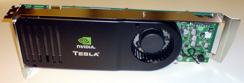NVIDIA Tesla GPU High‑performance GPU used for training deep neural networks (Image: Mahogny, Public domain, via Wikimedia Commons) 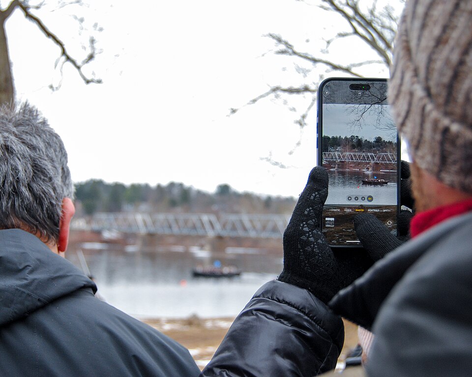Smartphone camera Input source for mobile CNN applications (Image: LR.127, CC BY 4.0, via Wikimedia Commons) 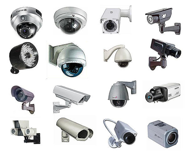CCTV camera Video feed processed by CNNs for surveillance (Image: Tamasflex, CC BY-SA 3.0, via Wikimedia Commons)

Exam tip

Diagram questions: Be ready to draw a 3‑layer MLP, label inputs, weights, biases, activations, and loss.
Back‑prop calculations: Practice computing $δ$ values for a small network; remember the chain rule and activation derivatives.
Comparisons: Know the key differences between perceptron, MLP, CNN, RNN, and GAN in terms of architecture, training, and use‑cases.
Applications: Relate each architecture to a real product (e.g., CNN → image search, RNN → language model).

Good luck!

Based on the TU BITM syllabus for Artificial Intelligence (IT228), unit 8.

Discussion

Loading…