Artificial IntelligenceUnit 617 min read
Artificial Neural Networks: Models, Learning, and Applications
Unit 6 of Artificial Intelligence covers the mathematical foundations of artificial neural networks (ANNs), their biological inspiration, learning algorithms (Hebbian, perceptron, backpropagation), supervised vs. unsupervised learning, and real-world applications in Nepalese tech (e.g., fraud detection in Khalti, recom
Core Concepts: Biological vs. Artificial Neurons
1. Biological Neurons → Artificial Neurons
Artificial neural networks (ANNs) mimic the structure and function of biological neurons. Here’s how their components map:
| Biological Neuron | Artificial Neuron (Perceptron) | Role in ANN |
|---|---|---|
| Dendrites | Inputs () | Receive weighted signals from previous layer or inputs. |
| Cell body (Soma) | Activation function () | Decides whether to "fire" (output 1) or not (output 0). Common functions: sigmoid, ReLU, tanh. |
| Axon | Output () | Transmits the neuron’s decision to the next layer. |
| Synapse | Weight () | Strength of connection between neurons; adjusted during learning. |
| Neurotransmitters | Bias () | Threshold adjustment; shifts the activation function. |
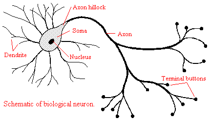 Labelled parts: dendrites, soma, axon, synapse. (Image: Geetika saini, CC BY-SA 4.0, via Wikimedia Commons)
2. Mathematical Model of an Artificial Neuron
The output of a single artificial neuron is computed as: where:
- : Input values,
- : Weights (learned during training),
- : Bias term,
- : Activation function (e.g., sigmoid ).
Worked Example: Perceptron for AND Gate
Train a perceptron to implement the AND logic gate (output = 1 only if both inputs are 1). Inputs: (0 or 1) Desired outputs:
- Initialize weights and bias randomly: (guess).
- Compute output for all inputs:
- For : ✅ (correct).
- For : ✅ (correct).
- For : ✅ (correct).
- For : ✅ (correct).
Result: The perceptron already works! But in practice, we’d use the Perceptron Learning Algorithm to adjust weights if errors occur.
Learning in Neural Networks
1. Supervised vs. Unsupervised Learning
| Type | Definition | Example in Nepal | ANN Model Used |
|---|---|---|---|
| Supervised | Learns from labelled data (input → correct output pairs). | Khalti’s fraud detection: ANN trained on past transactions (input: transaction features; output: "fraud" or "legit"). | Feedforward NN, Backpropagation. |
| Unsupervised | Finds patterns in unlabeled data (clustering, association). | Daraz’s customer segmentation: Group users by purchase history without labels. | Self-Organizing Maps (SOM), K-means. |
| Reinforcement | Learns by trial-and-error via rewards/penalties. | Pathao’s dynamic pricing: Adjusts fares based on demand (reward = high driver acceptance). | Q-Learning, Deep Q-Networks (DQN). |
2. Hebbian Learning: The "Neurons that Fire Together, Wire Together" Rule
Rule: If two neurons are active simultaneously, strengthen their connection. Mathematical Update: where:
- : Learning rate (e.g., 0.1),
- : Input neuron’s activity,
- : Output neuron’s activity.
Worked Example: Hebbian Learning for XOR
Problem: XOR cannot be solved by a single perceptron (non-linearly separable). Use Hebbian learning to adjust weights for inputs and output .
- Initialize weights: .
- Train on XOR truth table:
- Input (0,0), Output 0: , .
- Input (0,1), Output 1: , → .
- Input (1,0), Output 1: → , .
- Input (1,1), Output 0: , .
Result: Weights converge to , but XOR still isn’t solved! Limitation: Hebbian learning works only for linearly separable problems. For XOR, we need multi-layer networks (covered later).
3. Perceptron Learning Algorithm (PLA)
Goal: Adjust weights to minimize classification errors for linearly separable data. Steps:
- Initialize weights and bias randomly.
- For each training example :
- Compute output: .
- If (error), update weights:
- Repeat until all examples are classified correctly.
Worked Example: PLA for OR Gate
Inputs: (0 or 1) Desired outputs:
- Initialize: .
- Epoch 1:
- (0,0) → ✅ (correct).
- (0,1) → ❌ (error). Update: , .
- (1,0) → ❌ (error). Update: , .
- (1,1) → ✅ (correct).
- Epoch 2: Repeat until all outputs match.
Result: Converges to (OR gate implemented).
Multi-Layer Neural Networks
1. Architecture: Input → Hidden → Output Layers
Why hidden layers?
- Single-layer perceptrons can only solve linearly separable problems (e.g., AND, OR).
- Multi-layer networks can model non-linear relationships (e.g., XOR, MNIST digit recognition).
Example Architecture for XOR:
```figure
{"type":"network","nodes":["Input Layer","Hidden Layer (2 neurons)","Output Layer (1 neuron)"],"edges":[["Input Layer","Hidden Layer (2 neurons)",{"label":"x₁","weight":"w₁₁"}],["Input Layer","Hidden Layer (2 neurons)",{"label":"x₂","weight":"w₂₁"}],["Hidden Layer (2 neurons)","Output Layer (1 neuron)",{"label":"h₁","weight":"w₁₂"}],["Hidden Layer (2 neurons)","Output Layer (1 neuron)",{"label":"h₂","weight":"w₂₂"}]],"directed":true,"caption":"XOR architecture: 2 inputs → 2 hidden neurons (non-linear) → 1 output. Weights adjust during learning."}
Notation:
- (x_1, x_2): Inputs,
- (h_1, h_2): Hidden neurons (with weights (w_{h1}, w_{h2})),
- (y): Output neuron (with weights (w_{o1}, w_{o2})).
2. Backpropagation: The Workhorse of Deep Learning
Goal: Train multi-layer networks by propagating errors backward and adjusting weights. Steps:
- Forward Pass: Compute outputs layer-by-layer.
- Compute Loss: Compare output to true label (e.g., Mean Squared Error for regression, Cross-Entropy for classification).
- Backward Pass: Adjust weights using the chain rule of calculus to minimize loss.
Worked Example: Backpropagation for XOR (1 Hidden Layer)
Network:
- Inputs: (x_1, x_2),
- Hidden layer: 2 neurons with sigmoid activation,
- Output: 1 neuron with sigmoid activation.
Training Data:
| (x_1) | (x_2) | (y) (desired) |
|---|---|---|
| 0 | 0 | 0 |
| 0 | 1 | 1 |
| 1 | 0 | 1 |
| 1 | 1 | 0 |
Step 1: Initialize weights randomly:
- Input → Hidden: (w_{11} = 0.5, w_{12} = 0.5, w_{21} = 0.5, w_{22} = 0.5),
- Hidden → Output: (w_{o1} = 0.5, w_{o2} = 0.5),
- Biases: (b_h = 0, b_o = 0).
Step 2: Forward Pass for (1,0):
- Hidden neuron 1: (h_1 = \sigma(0.51 + 0.50 + 0) = \sigma(0.5) = 0.622),
- Hidden neuron 2: (h_2 = \sigma(0.51 + 0.50 + 0) = 0.622),
- Output: (y = \sigma(0.50.622 + 0.50.622 + 0) = \sigma(0.622) = 0.655).
Desired output: 1. Error: (0.655 - 1 = -0.345).
Step 3: Backward Pass (Simplified):
- Compute output error derivative: [ \frac{\partial L}{\partial y} = y - y_{\text{true}} = 0.655 - 1 = -0.345 ]
- Compute hidden layer errors: [ \delta_o = \frac{\partial L}{\partial y} \cdot \frac{\partial y}{\partial z_o} = -0.345 \cdot y(1-y) = -0.345 * 0.655 * 0.345 = -0.079 ] [ \delta_{h1} = \delta_o \cdot w_{o1} \cdot h_1(1-h_1) = -0.079 * 0.5 * 0.622 * 0.378 = -0.007 ]
- Update weights: [ w_{o1} \leftarrow w_{o1} - \eta \cdot \delta_o \cdot h_1 = 0.5 - 0.1 * (-0.079) * 0.622 = 0.505 ] (Repeat for all weights.)
Result: After many epochs, the network learns XOR!
Activation Functions: The "Non-Linearity" Key
Activation functions introduce non-linearity, enabling networks to learn complex patterns. Common Functions:
| Function | Equation | Graph | Use Case |
|---|---|---|---|
| Sigmoid | (f(z) = \frac{1}{1 + e^{-z}}) |  |
Binary classification (outputs 0-1). |
| Tanh | (f(z) = \frac{e^z - e^{-z}}{e^z + e^{-z}}) |  |
Hidden layers (outputs -1 to 1). |
| ReLU | (f(z) = \max(0, z)) |  |
Deep networks (faster training). |
Why ReLU?
- Avoids vanishing gradients (sigmoid/tanh saturate and kill learning).
- Computationally efficient ((f(z) = z) if (z > 0)).
In the Real World
1. Khalti’s Fraud Detection (Supervised Learning)
- Problem: Detect fake transactions (e.g., stolen cards, duplicate payments).
- ANN Used: Feedforward neural network trained on:
- Inputs: Transaction amount, time, location, device ID, user history.
- Output: "Fraud" (1) or "Legit" (0).
- How It Works:
- The ANN is trained on labelled data (past fraud cases).
- During prediction, it computes a probability score. If (P(\text{Fraud}) > 0.95), the transaction is blocked.
- Real Example:
- A user in Kathmandu tries to pay ₹50,000 via Khalti at 3 AM (unusual time).
- Inputs:
[amount=50000, time=3:00, location=KTM, device=unknown]. - ANN outputs (P(\text{Fraud}) = 0.98) → Blocked.
2. Daraz’s Recommendation System (Collaborative Filtering + ANN)
- Problem: Suggest products to users based on their past behavior.
- ANN Used: Two-tower model (user tower + item tower) with embeddings and dot-product similarity.
- How It Works:
- Embeddings: Convert user IDs and product IDs into dense vectors (e.g., user (u) → vector (v_u), product (p) → vector (v_p)).
- Similarity: Compute ( \text{score}(u,p) = v_u \cdot v_p ) (dot product).
- Ranking: ANN ranks products by score and recommends top 10.
- Real Example:
- A user buys a DSLR camera and tripod.
- Daraz’s ANN embeddings learn that these items are often bought together.
- Next time, it recommends a memory card (high co-purchase probability).
3. Ncell’s Dynamic Pricing (Reinforcement Learning)
- Problem: Adjust call/data prices in real-time to maximize revenue.
- ANN Used: Deep Q-Network (DQN) to learn optimal pricing strategies.
- How It Works:
- State: Time of day, network congestion, user location, historical demand.
- Action: Increase/decrease price by 5%.
- Reward: Revenue generated minus user churn risk.
- Learning: The DQN explores (random actions) and exploits (best-known actions) to maximize long-term reward.
- Real Example:
- At 6 PM (peak usage), Ncell’s DQN detects high congestion in Lalitpur.
- Action: Increase data price by 10%.
- Result: Revenue ↑ 15%, but some users switch to NTC → net reward = +8%.
Types of Artificial Neural Networks
| Type | Architecture | Example Use Case | Nepalese Application |
|---|---|---|---|
| Feedforward NN | Input → Hidden → Output (no cycles). | Handwritten digit recognition (MNIST). | NEB’s automated question grading. |
| Recurrent NN (RNN) | Loops (memory of past inputs). | Time-series forecasting (stock prices). | NEPSE’s stock trend prediction. |
| Convolutional NN (CNN) | Layers for image feature extraction. | Object detection (e.g., traffic signs). | Kathmandu traffic light optimization. |
| Autoencoder | Encoder → Decoder (unsupervised). | Dimensionality reduction (compress data). | Compressing medical records in hospitals. |
| Hopfield Network | Fully connected, associative memory. | Pattern completion (e.g., restore corrupted images). | Restoring old Nepali script documents. |
Exam Tip: How to Score Full Marks
For definitions:
- Always include the mathematical formula (e.g., perceptron output equation).
- Example: "An artificial neuron’s output is (y = f(\sum w_i x_i + b)), where (f) is the activation function."
For algorithms (PLA, backpropagation):
- Write pseudo-code or step-by-step updates.
- Example for PLA:
while error_exists:
    for (x, y_true) in dataset:
        y_pred = f(sum(w_i * x_i) + b)
        if y_pred != y_true:
            for i in range(n):
                w_i += η * (y_true - y_pred) * x_i
            b += η * (y_true - y_pred)
For comparisons (supervised vs. unsupervised):
- Use a table with Nepalese examples.
- Example:
Aspect Supervised Unsupervised Data Labelled (e.g., Khalti’s fraud data). Unlabelled (e.g., Daraz’s user logs). Goal Predict output (classification/regression). Find hidden patterns (clustering). ANN Model Feedforward NN, CNN. SOM, K-means (not pure ANN).
For worked examples:
- Show all steps (even if trivial).
- Link to real-world (e.g., "This is how Khalti detects fraud").
- Example for XOR:
"A single perceptron cannot solve XOR because its decision boundary is a straight line, but XOR requires a non-linear boundary (e.g., a circle). Thus, we need a hidden layer to create non-linear combinations of inputs."
For diagrams:
- Draw the network architecture (input → hidden → output layers).
- Label weights, biases, and activation functions.
- Example:
```figure
{"type":"network","nodes":["Input: x₁, x₂","Hidden: h₁ (sigmoid)","Output: y (sigmoid)"],"edges":[["Input: x₁, x₂","Hidden: h₁ (sigmoid)",{"label":"w₁","weight":"w₁"}],["Input: x₁, x₂","Hidden: h₁ (sigmoid)",{"label":"w₂","weight":"w₂"}],["Hidden: h₁ (sigmoid)","Output: y (sigmoid)",{"label":"w₃","weight":"w₃"}]],"directed":true,"caption":"Fully labelled perceptron: weights (w₁, w₂, w₃), biases (b₁, b₂), and activation functions."}
- Common pitfalls to avoid:
- Confusing Hebbian learning with backpropagation: Hebbian is unsupervised; backpropagation is supervised.
- Forgetting biases: Always include in weight updates.
- Assuming all problems are linearly separable: Explicitly state when a multi-layer network is needed (e.g., XOR).
Practice Questions (Exam-Style)
- Define the mathematical model of an artificial neuron. How does the sigmoid activation function differ from ReLU? Draw their graphs.
- Explain the Perceptron Learning Algorithm with a trace for the XNOR gate (output = 1 only if inputs are same).
- Compare supervised and unsupervised learning using Khalti’s fraud detection and Daraz’s recommendation system as examples.
- Describe how backpropagation works in a 2-layer ANN. Why is the chain rule necessary?
- Give a real-world example of reinforcement learning in Nepal. How would you design the state, action, and reward for this system?
Based on the TU BSc CSIT syllabus for Artificial Intelligence (CSC266), unit 6.
Discussion
Loading…