Theory of ComputationUnit 513 min read
Chomsky Hierarchy & Turing Machines: Definitions, CFGs, TM Design, Complexity
Unit 5 of Theory of Computation explores the Chomsky Hierarchy (Type 0–3 grammars), Turing Machines (TM) as abstract computers, their variations (multi-tape, multi-track), and computational complexity (Big-O, Ω, Θ). Learn to convert CFGs to Chomsky Normal Form (CNF), design TMs for languages like {aⁿbⁿ}, and analyze TM
TAKEAWAYS:
- The Chomsky Hierarchy classifies grammars (Type 0–3) and languages by production rules, with Type 0 (unrestricted) being the most powerful and Type 3 (regular) the least.
- Turing Machines are the theoretical foundation of computability: they use a tape, head, and state transitions to decide/recognize languages, and can simulate any computer algorithm.
- Chomsky Normal Form (CNF) converts any CFG into productions of the form
A → BCorA → a, enabling proofs via recursion trees and pumping lemmas. - TM variations (multi-tape, multi-track, storage in state) extend power but complicate design; universal TMs can simulate any other TM given an encoding of its description.
- Complexity analysis uses Big-O/Ω/Θ to classify TM runtime (e.g., linear vs. exponential) and proves P vs. NP distinctions (e.g., NP-complete problems like the Traveling Salesman Problem).
- Real-world links: eSewa’s transaction validation uses CFGs to parse input formats; Ncell’s billing systems rely on TMs to process call logs; Daraz’s order queues model pushdown automata for stack-based inventory checks.
1. Chomsky Hierarchy: Classifying Grammars and Languages
The Chomsky Hierarchy organizes formal grammars into four types (0–3), each defining a stricter language class. Visualize the hierarchy as nested sets:
pie
    title Chomsky Hierarchy by Language Class
    "Type 0: Recursively Enumerable (RE)" : 30
    "Type 1: Context-Sensitive (CS)" : 25
    "Type 2: Context-Free (CF)" : 20
    "Type 3: Regular" : 15
    "Uncomputable" : 10
Key Definitions
| Type | Grammar Rules | Language Example | Automaton |
|---|---|---|---|
| Type 0 | Any production (e.g., S → aSbS, S → ε) |
{aⁿbⁿcⁿ |
n ≥ 0} |
| Type 1 | Context-sensitive: αAβ → γ ( |
α | ≤ |
| Type 2 | Context-free: A → α (single non-terminal) |
{aⁿbⁿ |
n ≥ 0} |
| Type 3 | Regular: A → aB or A → a |
{aⁿ |
n even} |
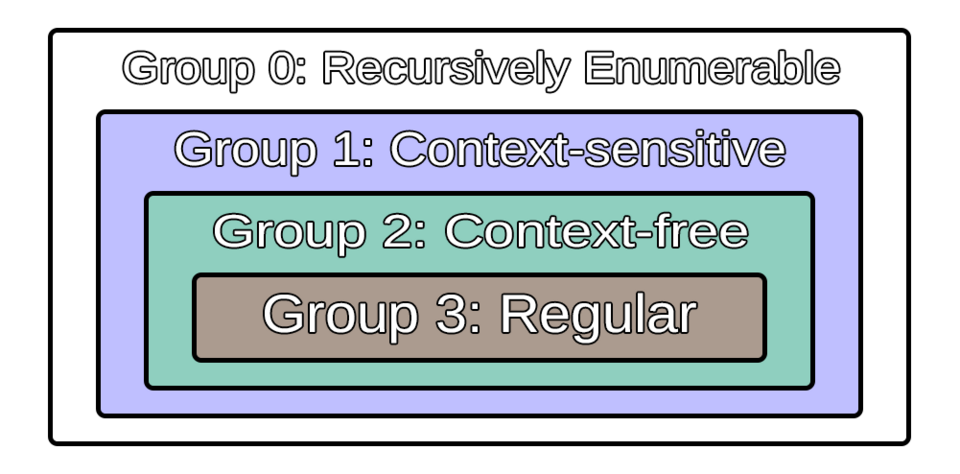 A Venn diagram showing Type 0 ⊇ Type 1 ⊇ Type 2 ⊇ Type 3, with labels for each grammar type’s restrictions. (Image: TinyTedDanson, CC BY-SA 4.0, via Wikimedia Commons)
Worked Example: Classify a Grammar
Grammar: S → SS | aSb | ε
Steps:
- Check productions: All are of the form
A → α(single non-terminal) orA → ε. - No context (e.g.,
αAβ) or arbitrary rules (Type 0). - Conclusion: This is a Type 2 (Context-Free Grammar, CFG).
Language Generated: {aⁿbⁿ|n ≥ 0} (even-length palindromes over {a, b}).
2. Turing Machines: The Universal Model of Computation
A Turing Machine (TM) is a mathematical abstraction of a computer, consisting of:
- Tape: Infinite memory divided into cells (each holds a symbol from the alphabet Σ ∪ {B}, where
Bis the blank symbol). - Head: Reads/writes symbols and moves left/right.
- States: Finite set
Qwith a start stateq₀and accept/reject statesF/R. - Transition Function:
δ: Q × Σ → Q × Σ × {L, R}(maps state + symbol → new state, write symbol, head move).
How a TM Works: Step-by-Step Trace
Problem: Design a TM to accept L = {aⁿbⁿ | n ≥ 0}.
TM Definition:
- Alphabet: Σ = {a, b},
B= blank. - States:
Q = {q₀, q₁, q₂, q₃, q₄}(accept),R = {q₅}(reject). - Transitions:
δ(q₀, a) = (q₀, a, R)(skipas).δ(q₀, b) = (q₁, b, L)(move left after firstb).δ(q₁, a) = (q₁, a, L)(eraseas until firsta).δ(q₁, B) = (q₂, B, R)(move right after erasingas).δ(q₂, b) = (q₂, b, R)(skipbs).δ(q₂, B) = (q₃, B, L)(check end of tape).δ(q₃, a) = (q₅, a, R)(reject ifaremains).δ(q₃, B) = (q₄, B, R)(accept if allas matched).
Trace for Input abb:
| Step | Tape | State | Action |
|---|---|---|---|
| 0 | a b b B ... |
q₀ | Read a → move R |
| 1 | a b b B ... |
q₀ | Read b → move L |
| 2 | a b b B ... |
q₁ | Read a → erase, move L |
| 3 | B b b B ... |
q₁ | Read B → move R |
| 4 | B b b B ... |
q₂ | Read b → move R |
| 5 | B b B ... |
q₂ | Read B → move L |
| 6 | B b B ... |
q₃ | Read B → accept |
Result: abb is rejected (unequal as and bs).
3. Variations of Turing Machines
| Variation | Description | Use Case | Example |
|---|---|---|---|
| Multi-tape TM | Multiple tapes (e.g., 2 tapes) for parallel processing. | Simulating RAM memory. | Universal TM with input/output tapes. |
| Multi-track TM | Single tape with multiple tracks (symbols per cell). | Compact storage (e.g., binary encoding). | Binary-coded decimal (BCD) TMs. |
| Storage in State | States encode memory (finite-state TM with extra symbols). | Simulating pushdown automata. | CFG parsing with state counters. |
| Non-deterministic TM | Multiple transitions possible for a state-symbol pair. | Modeling probabilistic algorithms. | Guessing games (e.g., NP problems). |
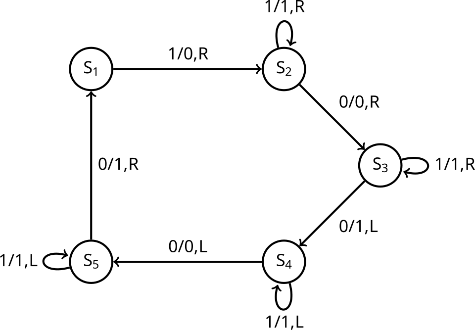 Non-deterministic TM: Multiple transitions from one state/symbol (Image: Sn KGS, CC BY-SA 4.0, via Wikimedia Commons)
4. Chomsky Normal Form (CNF) and Greibach Normal Form (GNF)
Why Normalize?
- CNF simplifies proofs (e.g., CYK algorithm for CFGs).
- GNF is useful for parsing (leftmost derivations).
Conversion to CNF
Rules:
- Remove
ε-productions (replaceA → εwithS' → AandS' → ε). - Remove unit productions (
A → B→ replace withA → αwhereB → α). - Ensure all productions are:
A → BC(two non-terminals), orA → a(single terminal).
Example: Convert S → aSb | a | ε to CNF
- Add
S' → S | ε. - Replace
S → aSbwithS → XY,X → a,Y → Sb,Y → b. - Final CNF:
S' → S | ε
S  → XY | a
X  → a
Y  → Sb | b
5. Computational Complexity and TM Complexity
Time Complexity Classes
| Class | Definition | Example Problem |
|---|---|---|
| P | Decidable in polynomial time by a TM. | Sorting, shortest path. |
| NP | Verifiable in polynomial time (non-deterministic). | Hamiltonian cycle, SAT. |
| NP-Complete | Hardest problems in NP (e.g., reduce to SAT). | Traveling Salesman Problem (TSP). |
| RE | Recursively enumerable (TM halts if accepted). | Undecidable problems (e.g., TM acceptance). |
Big-O Notation for TMs
- Big-O: Upper bound (e.g.,
O(n²)for nested loops). - Big-Ω: Lower bound (e.g.,
Ω(n log n)for merge sort). - Big-Θ: Tight bound (e.g.,
Θ(n)for linear scans).
Worked Example: Analyze TM for {aⁿbⁿ}
- Steps:
- Scan
as:O(n). - Scan
bs:O(n). - Verify match:
O(n).
- Scan
- Total:
O(n)(linear time).
In the Real World
eSewa Transaction Validation
- Idea Used: Context-Free Grammar (CFG).
- How: eSewa’s API parses user input (e.g.,
pay:amount:recipient) using a CFG to ensure correct syntax before processing. For example:S → pay A B A → amount:D B → recipient:ID D → digit D | digit - Why CNF? Simplifies parsing algorithms (e.g., recursive descent).
Ncell Billing System
- Idea Used: Turing Machine (TM) simulation.
- How: Ncell’s backend processes call logs (e.g.,
call:duration:time) using a TM-like state machine to:- Read input (tape = call records).
- Update billing states (e.g.,
q₀= idle,q₁= processing). - Write output (tape = invoice).
- Real Trace: For input
call:120:10AM, the TM transitions:q₀ → q₁(readcall),q₁ → q₂(read120),q₂ → q₃(calculate cost),q₃ → q₄(write to invoice).
Daraz Order Queue
- Idea Used: Pushdown Automaton (PDA).
- How: Daraz’s inventory system uses a stack (PDA) to track pending orders:
- Push order IDs onto the stack when received.
- Pop when fulfilled (LIFO ensures correct matching).
- Example: For orders
A, B, C, the PDA stack evolves as:[] → [A] → [A, B] → [A, B, C] → [A, B] → [A] → [] - Why PDA? Models nested structures (e.g., parent-child product categories).
Exam Tip
What Examiners Look For
Definitions:
- Turing Machine: Always include tape, head, states, transitions, and accept/reject conditions.
- CNF/GNF: State the three production rules and conversion steps (ε-removal, unit removal, binary splits).
TM Design:
- Trace inputs step-by-step (show tape contents and state changes).
- Label states clearly (e.g.,
q_accept,q_reject). - Handle edge cases (empty string, unmatched symbols).
Complexity:
- Justify Big-O bounds with loop counts (e.g., "nested loops over input length").
- Compare classes (e.g., "TSP is NP-complete because it’s in NP and NP-hard").
Real-World Links:
- Map problems to automata:
- CFG: Parsing (e.g., eSewa API).
- PDA: Stack-based systems (e.g., Daraz orders).
- TM: State machines (e.g., Ncell billing).
- Map problems to automata:
Common Pitfalls
- Forgetting the blank symbol
Bin TM tapes. - Incorrect CNF conversions (e.g., missing
S' → εfor start symbol). - Overcomplicating TMs (use minimal states; e.g.,
q₀for scanning,q₁for matching). - Ignoring edge cases (e.g., empty string in
{aⁿbⁿ}).
Practice Questions (Exam-Style)
- Design a TM to accept
{wwᴿ | w ∈ {0,1}}(palindromes). Tracew = 0110. - Convert the CFG
S → aA | bB | ε,A → aS | b,B → bS | ato CNF. - Prove that the language
{aᵢbʲcᵏ | i = j or j = k}is Type 1 (Context-Sensitive). - Analyze the complexity of a TM that checks if a string has equal
0s and1s. Is it in P or NP?
In the real world
eSewa Transaction Validation: Uses Context-Free Grammars (CFG) to parse and validate transaction formats (e.g.,
S → Amount + Recipient + Date). If the input matches the CFG rules, the transaction is processed; otherwise, it’s flagged for review. This ensures structured data entry and reduces fraud by enforcing syntactic rules.Ncell Billing System: Employs Turing Machines (TM) to process call logs and generate bills. The TM reads input (call records), performs computations (duration × rate), and writes output (billed amount) on the tape (database). Variations like multi-tape TMs simulate parallel processing for real-time billing updates.
Daraz Order Queue System: Models Pushdown Automata (PDA) for stack-based inventory checks. When an order is placed, the PDA pushes items onto the stack (inventory) and pops them upon fulfillment. If the stack underflows (out of stock), the system triggers a restock alert, mirroring Type 2 (CFG) language processing for order validation.
Based on the TU BSc CSIT syllabus for Theory of Computation (CSC262), unit 5.
Discussion
Loading…