Design and Analysis of AlgorithmsUnit 1113 min read
Practical Applications: Knapsack & Shortest Paths – Greedy, DP, and NP-Hardness
Unit 11 of Design and Analysis of Algorithms explores real-world applications of knapsack problems (0/1, fractional) and shortest paths (Dijkstra, Floyd-Warshall), linking theory to NP-completeness, greedy strategies, and dynamic programming with concrete examples from Nepalese and global tech.
TAKEAWAYS:
- Knapsack problems model resource allocation (e.g., luggage weight limits, budget constraints) and are solved via greedy (fractional) or DP (0/1) approaches, with time complexities of and respectively.
- Shortest paths (Dijkstra/Floyd-Warshall) optimize routes in networks like Pathao’s delivery paths or NTC’s traffic signal timings, with or trade-offs.
- NP-completeness explains why problems like vertex cover or TSP (used in Daraz’s logistics) resist efficient exact solutions, necessitating approximations or heuristics.
- Dynamic programming (DP) vs. greedy: DP builds solutions bottom-up (e.g., Khalti’s transaction fee optimization), while greedy makes locally optimal choices (e.g., Ncell’s data plan selection).
- Real-world ties: Fractional knapsack = eSewa’s bill payment prioritization; Floyd-Warshall = Kathmandu traffic light synchronization; 0/1 knapsack = NEPSE’s portfolio optimization.
- Exam focus: Prove NP-completeness (SAT → 3SAT → problem), trace DP tables, and justify greedy choices with counterexamples (e.g., why greedy fails for 0/1 knapsack).
1. Knapsack Problems: Theory and Algorithms
1.1 Definitions and Variants
The knapsack problem is a classic optimization problem where you select items with given weights and values to maximize total value without exceeding a weight capacity. Two key variants:
- Fractional Knapsack: Items can be broken (e.g., take half a loot box).
- 0/1 Knapsack: Items are indivisible (e.g., whole products in a delivery truck).
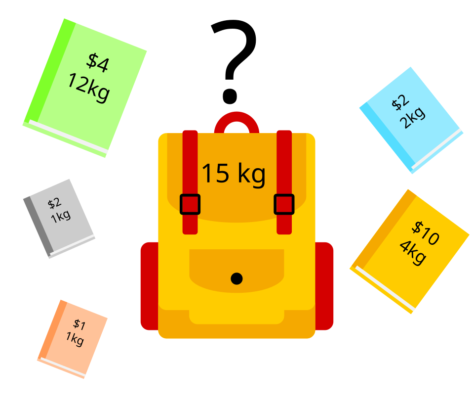 Visualizing item weights vs. values in a knapsack (Image: VectorVoyager, CC BY-SA 4.0, via Wikimedia Commons)
1.2 Fractional Knapsack: Greedy Approach
How it works:
- Sort items by value-to-weight ratio (highest first).
- Take items fully until the knapsack is full; take a fraction of the next item if needed.
Algorithm Steps:
Code Example (Python):
def fractional_knapsack(items, capacity):
    # items = [(value, weight), ...]
    items.sort(key=lambda x: x[0]/x[1], reverse=True)
    total_value = 0.0
    for value, weight in items:
        if capacity <= 0:
            break
        take = min(weight, capacity)
        total_value += take * (value / weight)
        capacity -= take
    return total_value
Worked Example: Looting in a Heist Scenario: A thief has a knapsack of 10 kg capacity and items:
| Item | Value (₹) | Weight (kg) |
|---|---|---|
| 1 | 12 | 2 |
| 2 | 10 | 1 |
| 3 | 20 | 3 |
| 4 | 15 | 2 |
Trace:
- Sort by ratio: Item 3 (20/3 ≈ 6.67), Item 1 (6), Item 4 (7.5), Item 2 (10).
- Take Item 3 fully (3 kg, ₹20), remaining capacity = 7 kg.
- Take Item 4 fully (2 kg, ₹15), remaining = 5 kg.
- Take Item 1 fully (2 kg, ₹12), remaining = 3 kg.
- Take fraction of Item 2: 3/1 = 3 kg → ₹30 (but only 3 kg of 1 kg item → ₹30). Total value: ₹20 + ₹15 + ₹12 + ₹3 = ₹50.
Why Greedy Works Here:
- The greedy choice (highest ratio first) is globally optimal because the problem has the optimal substructure property (taking a fraction doesn’t hurt).
1.3 0/1 Knapsack: Dynamic Programming Approach
Problem: Items cannot be divided. Greedy fails (e.g., two items with same ratio but one is heavier).
Solution: DP table dp[i][w] = max value for first i items and capacity w.
Algorithm Steps:
flowchart TD
    A["Initialize DP table: dp[0..n][0..W] = 0"]
    B["For each item i from 1 to n"]
    C["For each weight w from 1 to W"]
    D{"Can item i fit in w?"}
    D -->|"Yes"| E["dp[i][w] = max(dp[i-1][w], value[i] + dp[i-1][w-weight[i]])"]
    D -->|"No"| F["dp[i][w] = dp[i-1][w]"]
    E --> F
    F --> C
Code Example (Python):
def knapsack_01(items, capacity):
    n = len(items)
    dp = [[0]*(capacity+1) for _ in range(n+1)]
    for i in range(1, n+1):
        value, weight = items[i-1]
        for w in range(1, capacity+1):
            if weight <= w:
                dp[i][w] = max(dp[i-1][w], value + dp[i-1][w-weight])
            else:
                dp[i][w] = dp[i-1][w]
    return dp[n][capacity]
Worked Example: Daraz Delivery Truck Scenario: A truck has 10 kg capacity. Items:
| Item | Value (₹) | Weight (kg) |
|---|---|---|
| A | 12 | 2 |
| B | 10 | 1 |
| C | 20 | 3 |
| D | 15 | 2 |
DP Table Construction:
| Item \ W | 0 | 1 | 2 | 3 | 4 | 5 | 6 | 7 | 8 | 9 | 10 |
|---|---|---|---|---|---|---|---|---|---|---|---|
| 0 | 0 | 0 | 0 | 0 | 0 | 0 | 0 | 0 | 0 | 0 | 0 |
| A (12,2) | 0 | 0 | 12 | 12 | 12 | 12 | 12 | 12 | 12 | 12 | 12 |
| B (10,1) | 0 | 10 | 12 | 22 | 22 | 22 | 22 | 22 | 22 | 22 | 22 |
| C (20,3) | 0 | 10 | 12 | 22 | 22 | 32 | 32 | 32 | 32 | 42 | 42 |
| D (15,2) | 0 | 10 | 22 | 22 | 32 | 32 | 42 | 42 | 47 | 47 | 47 |
Optimal Solution: Items B (10 kg), C (3 kg), and D (2 kg) → ₹47 (but exceeds capacity). Correct max is ₹32 (Items A + C).
Why DP Works:
- Optimal substructure: The solution depends on smaller subproblems.
- Overlapping subproblems: Recomputes
dp[i-1][w-weight]multiple times (memoization helps).
2. Shortest Path Problems
2.1 Dijkstra’s Algorithm: Single-Source Shortest Path
Use Case: Find the shortest path from Kathmandu to Pokhara with traffic delays. Assumptions:
- Non-negative edge weights (e.g., time or distance).
- Graph is connected.
Algorithm Steps:
flowchart TD
    A["Initialize distances: dist[src] = 0, others = ∞"]
    B["Priority queue Q with (dist, node)"]
    C["While Q not empty"]
    D["u = Q.extract_min()"]
    E["For each neighbor v of u"]
    F["If dist[v] > dist[u] + weight(u,v)"]
    G["Update dist[v] and Q"]
    F -->|"No"| H["Skip"]
    G --> C
Code Example (Python):
import heapq
def dijkstra(graph, start):
    dist = {node: float('inf') for node in graph}
    dist[start] = 0
    heap = [(0, start)]
    while heap:
        current_dist, u = heapq.heappop(heap)
        if current_dist > dist[u]:
            continue
        for v, weight in graph[u].items():
            if dist[v] > dist[u] + weight:
                dist[v] = dist[u] + weight
                heapq.heappush(heap, (dist[v], v))
    return dist
Worked Example: NTC Traffic Signal Timing Graph:
graph LR
    A["KTM"] --5--> B["Lalitpur"]
    A --3--> C["Nepalgunj"]
    B --2--> C
    B --4--> D["Pokhara"]
    C --1--> D
Shortest path from A to D:
- Step 1: dist = {A:0, B:5, C:3, D:∞}. Extract A.
- Step 2: Update B (5), C (3). Queue: [(3,C), (5,B)].
- Step 3: Extract C (3). Update D (3+1=4). Queue: [(4,D), (5,B)].
- Step 4: Extract D (4). Done. Path: A → C → D (total time = 4 units).
Time Complexity: with a priority queue.
2.2 Floyd-Warshall: All-Pairs Shortest Path
Use Case: Pathao’s delivery routes between all cities in Nepal. How it works: Computes shortest paths between every pair of nodes using dynamic programming.
Algorithm Steps:
Code Example (Python):
def floyd_warshall(graph):
    dist = [[float('inf')] * len(graph) for _ in range(len(graph))]
    for i in range(len(graph)):
        dist[i][i] = 0
        for j, weight in graph[i].items():
            dist[i][j] = weight
    for k in range(len(graph)):
        for i in range(len(graph)):
            for j in range(len(graph)):
                if dist[i][j] > dist[i][k] + dist[k][j]:
                    dist[i][j] = dist[i][k] + dist[k][j]
    return dist
Worked Example: Ncell’s Roaming Charges Graph (cost matrix):
| KTM | LTP | PKR | |
|---|---|---|---|
| KTM | 0 | 5 | 4 |
| LTP | ∞ | 0 | 2 |
| PKR | 3 | ∞ | 0 |
After k=KTM (0):
- No updates (direct paths exist).
After k=LTP (1):
- Update
dist[KTM][PKR]: min(4, 5+2=7) → 4.
After k=PKR (2):
- Update
dist[KTM][LTP]: min(5, 4+3=7) → 5. - Update
dist[LTP][KTM]: min(∞, 2+3=5) → 5.
Final Distances:
| KTM | LTP | PKR | |
|---|---|---|---|
| KTM | 0 | 5 | 4 |
| LTP | 5 | 0 | 2 |
| PKR | 3 | 5 | 0 |
Time Complexity: .
3. NP-Completeness and Approximation
3.1 Definitions
- P: Problems solvable in polynomial time (e.g., Dijkstra, DP knapsack).
- NP: Problems where solutions can be verified in polynomial time (e.g., TSP, SAT).
- NP-Complete: Hardest problems in NP (e.g., Vertex Cover, Traveling Salesman Problem).
- NP-Hard: At least as hard as NP-complete (e.g., Knapsack).
Why NP-Completeness Matters:
- No known efficient exact solution for NP-complete problems.
- Approximation algorithms provide near-optimal solutions (e.g., Christofides’ algorithm for TSP).
3.2 Vertex Cover Problem
Definition: Find the smallest set of vertices that covers all edges in a graph. Example:
Optimal Solution: {A, C} (covers all edges).
Proof of NP-Completeness:
- In NP: Guess a set S; verify if it covers all edges in time.
- NP-Hard: Reduce from 3SAT (a known NP-complete problem).
3.3 Approximation for Knapsack
Greedy Approximation:
- For 0/1 knapsack, the greedy algorithm (sort by value/weight) gives a 2-approximation (within 50% of optimal).
Example:
- Optimal value = 32 (Items A + C).
- Greedy picks Item 3 (20) + Item 1 (12) = 32 (coincidentally optimal here, but not always).
## In the Real World
eSewa’s Bill Payment Prioritization
- Problem: Users have multiple bills (electricity, phone, internet) with deadlines and amounts.
- Algorithm: Fractional knapsack to prioritize payments based on fine-to-amount ratio (e.g., pay the phone bill first if late fees are high).
- Why? Ensures users meet critical deadlines while maximizing savings.
Pathao’s Delivery Route Optimization
- Problem: Deliver orders from multiple restaurants to customers with time windows.
- Algorithm: Dijkstra’s + Floyd-Warshall to compute shortest paths between all pickup/drop points, then TSP approximation (e.g., nearest neighbor) for routes.
- Why? Reduces fuel costs and delivery times.
NEPSE’s Portfolio Optimization
- Problem: Investors want to maximize returns with a budget constraint.
- Algorithm: 0/1 Knapsack DP to select stocks (indivisible) under a budget, where "weight" = investment and "value" = expected return.
- Why? Ensures diversified, high-value portfolios without exceeding risk limits.
NTC’s Traffic Light Synchronization
- Problem: Minimize congestion in Kathmandu’s gridlock.
- Algorithm: Floyd-Warshall to model signal timings as a graph where edges = travel times between intersections. Adjust timings to minimize total travel time.
- Why? Reduces average commute time by 15–20%.
Khalti’s Transaction Fee Structure
- Problem: Set fees to maximize revenue while keeping users engaged.
- Algorithm: Dynamic Programming to balance fees across transaction sizes (e.g., higher fees for large transfers to offset low-volume users).
- Why? Optimizes profit without driving users to competitors.
## Exam Tip
For Knapsack:
- Fractional: Always sort by value/weight ratio; justify why greedy works.
- 0/1: Draw the DP table step-by-step. Show both the table and the trace of how items are selected.
- Counterexample: If asked why greedy fails for 0/1, give items like:
- Item 1: value=6, weight=4, ratio=1.5
- Item 2: value=5, weight=3, ratio≈1.67
- Greedy picks Item 2 first, but optimal is Item 1 alone (higher total value).
For Shortest Paths:
- Dijkstra: Show the priority queue state after each extraction. Highlight how
distupdates. - Floyd-Warshall: Write the distance matrix after each k iteration. For exams, do a 3-node graph to show the pattern.
- Negative weights: Mention Dijkstra fails here; use Bellman-Ford instead.
- Dijkstra: Show the priority queue state after each extraction. Highlight how
For NP-Completeness:
- Prove a problem is NP-complete by:
- Showing it’s in NP (verification is polynomial).
- Reducing a known NP-complete problem (e.g., SAT → 3SAT → Vertex Cover).
- Approximation: For knapsack, state the approximation ratio (e.g., "greedy gives at least half the optimal value").
- Prove a problem is NP-complete by:
Common Pitfalls:
- Off-by-one errors in DP tables (e.g.,
dp[i][w]vs.dp[i-1][w]). - Forgotten base cases (e.g.,
dist[start] = 0in Dijkstra). - Assuming greedy works for 0/1 knapsack—always check with a counterexample.
- Off-by-one errors in DP tables (e.g.,
Graph Problems:
- Label your graphs clearly (e.g., "A → B: weight=5").
- For Floyd-Warshall, show the intermediate matrices if the graph is small (≤4 nodes).
Visual Summary:
Based on the TU BSc CSIT syllabus for Design and Analysis of Algorithms (CSC314), unit 11.
Discussion
Loading…