Image ProcessingUnit 28 min read
Image Formation & Representation: Pixels, Intensity, and Digital Encoding
Unit 2 of Image Processing: Explores how images are captured, digitized, and represented in digital systems, covering pixel intensity, spatial resolution, color models, and quantization—key concepts for processing and analyzing digital images.
TAKEAWAYS:
- Images are formed by capturing light intensity at discrete points called pixels, which are quantized into discrete intensity levels (gray or color).
- Digital representation involves converting continuous spatial and intensity domains into discrete matrices using sampling and quantization.
- Color models (RGB, HSV, YCbCr) define how pixels encode color, with each model serving different processing needs (e.g., YCbCr for compression).
- Resolution (spatial and intensity) determines image quality, where higher resolution means finer detail but larger file sizes.
- Noise and artifacts during formation (e.g., sensor noise, compression) degrade image quality and must be addressed in restoration.
- Image formats (JPEG, PNG, BMP) use different encoding schemes to balance quality, compression, and storage efficiency.
1. Image Formation: From Analog to Digital
1.1 Light and Sensor Interaction
- Light Intensity: Objects reflect or emit light at varying intensities, which the sensor measures.
- Sensor Types:
- CCD/CMOS Sensors: Common in digital cameras, they convert light into electrical signals.
- Medical Imaging: X-rays, MRIs, or CT scans capture internal structures using different sensors.
- Remote Sensing: Satellites capture Earth’s surface using multispectral sensors.
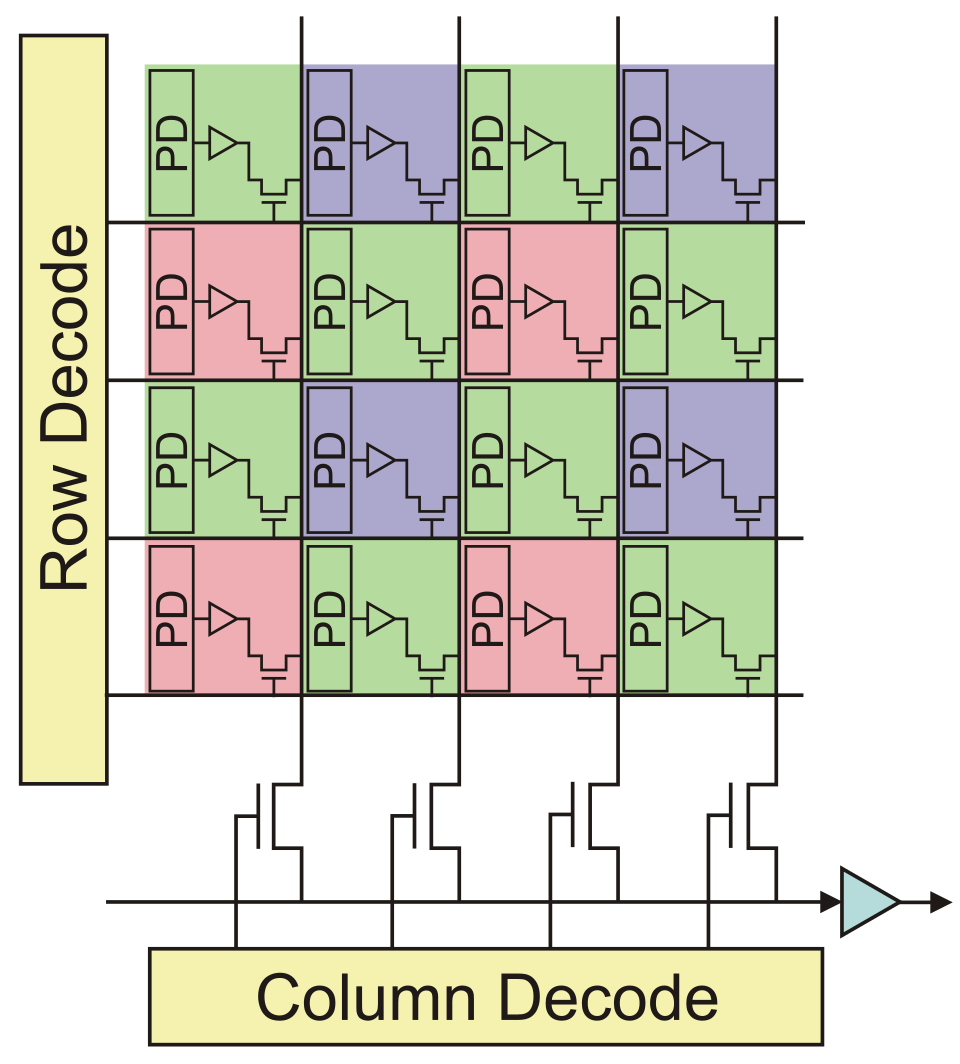 A CMOS sensor array converts incoming light into electrical signals via photodiodes. (Image: Shape, GPL, via Wikimedia Commons)
1.2 Sampling and Quantization
To digitize an image, we must:
- Sample the spatial domain: Divide the continuous image into discrete pixels (sampling).
- Quantize intensity levels: Assign discrete intensity values to each pixel (quantization).
flowchart LR
    A["Continuous Image"] -->|"Spatial Sampling"| B["Discrete Pixels (M×N)"]
B -->|"Intensity Quantization"| C["Digital Image (0 to L-1)"]- Sampling Theorem: To avoid aliasing, the sampling frequency must be at least twice the highest frequency in the image (Nyquist rate).
- Quantization: The number of discrete levels (e.g., 8-bit = 256 levels) affects image quality and file size.
2. Digital Image Representation
A digital image is represented as a matrix where each element corresponds to a pixel’s intensity. The matrix dimensions are:
- M × N: Spatial dimensions (rows × columns).
- L: Number of intensity levels (e.g., 256 for 8-bit grayscale).
2.1 Pixel Intensity
- Grayscale: Intensity values range from 0 (black) to (white).
- Color: Typically represented using RGB (Red, Green, Blue) or other models like HSV (Hue, Saturation, Value).
2.2 Color Models
Different color models serve different purposes:
| Model | Description | Use Case |
|---|---|---|
| RGB | Primary colors (Red, Green, Blue) combined additively. | Display devices (monitors, TVs). |
| HSV | Hue (color), Saturation (intensity), Value (brightness). | Color manipulation (e.g., hue rotation). |
| YCbCr | Luminance (Y) + Chrominance (Cb, Cr). | Video compression (e.g., JPEG). |
| CMYK | Cyan, Magenta, Yellow, Key (Black) for subtractive color mixing. | Printing. |
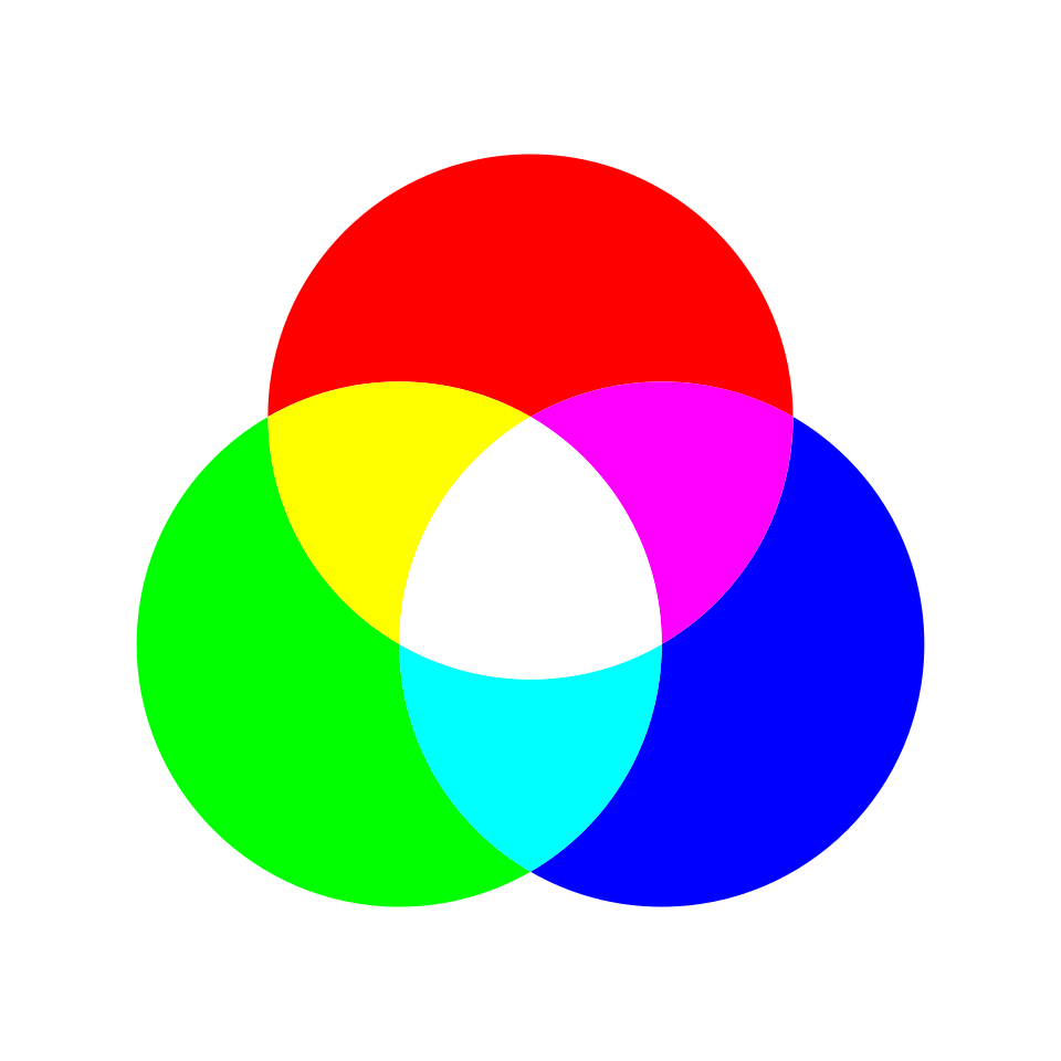 The RGB color cube shows how red, green, and blue combine to form colors. (Image: Youssef Abdelhamed, CC BY-SA 4.0, via Wikimedia Commons)
2.3 Bit Depth and Resolution
- Bit Depth: Number of bits per pixel (e.g., 8-bit = 256 levels, 16-bit = 65,536 levels).
- Spatial Resolution: Measured in pixels per inch (PPI) or dots per inch (DPI). Higher resolution = finer detail but larger file size.
3. Image Formation Models
- Object Scenes: The original scene (e.g., a landscape).
- Atmospheric Effects: Scattering, haze, or fog.
- Sensor Response: Noise, distortion, or quantization errors.
The degradation model can be represented as: where:
- : Degraded image (output).
- : Original image (input).
- : Point spread function (PSF) or blur kernel.
- : Noise.
- : Convolution operation.
3.1 Common Degradation Sources
| Source | Effect | Example |
|---|---|---|
| Motion Blur | Smearing due to relative motion between object and sensor. | Blurry photos in low light. |
| Defocus Blur | Uniform blur due to incorrect lens focus. | Soft, out-of-focus images. |
| Noise | Random variations in pixel intensity (e.g., salt-and-pepper, Gaussian). | Noisy medical scans. |
| Quantization | Loss of precision due to discrete intensity levels. | JPEG artifacts. |
4. Worked Example: Image Quantization
Problem: Given a continuous intensity range of 0 to 100, quantize it into 8-bit levels (0 to 255).
Solution:
- Range: 0 to 100 (101 levels).
- Quantization Step: .
- Mapped Levels:
- 0 → 0
- 10 →
- 50 →
- 100 → 255
5. Image Formats and Compression
Digital images are stored in formats like JPEG, PNG, or BMP, each with trade-offs:
| Format | Compression | Lossy? | Use Case |
|---|---|---|---|
| BMP | None | No | Uncompressed, high quality. |
| PNG | Lossless | No | Web graphics, transparency. |
| JPEG | Lossy | Yes | Photos, web images. |
| GIF | Lossless | No | Animated images, low color. |
Example: JPEG uses DCT (Discrete Cosine Transform) to compress images by discarding high-frequency components (less noticeable to the human eye).
6. In the Real World
eSewa/Khalti (Mobile Payments):
- Idea: Image-based OCR (Optical Character Recognition) is used to verify user IDs or bank statements uploaded via mobile apps.
- How: The app processes the image to extract text (e.g., account numbers) using digital image representation and segmentation techniques.
Daraz (E-commerce):
- Idea: Product Image Compression ensures fast loading of product images on mobile devices.
- How: JPEG compression reduces file size while maintaining visual quality, using frequency-domain analysis to discard less perceptible details.
NTC/Ncell (Telecom):
- Idea: Face Recognition for Unlocking Phones relies on digital image processing to capture and analyze facial features.
- How: The phone’s camera captures a grayscale or color image, which is then processed using pixel intensity analysis and feature extraction (e.g., edge detection) to match against stored templates.
7. Exam Tip
This unit is highly visual and often tested with:
- Definitions: Expect questions on pixel, quantization, color models, and degradation models.
- Mathematical Problems: Solve quantization, bit depth calculations, or simple convolution examples.
- Comparisons: Differentiate between RGB, HSV, and YCbCr; or spatial vs. frequency domain.
- Real-World Applications: Link concepts to apps (e.g., "How does Daraz compress images?").
- Diagrams: Always draw the degradation model equation or a color model cube if asked.
Common Pitfalls:
- Confusing sampling (spatial) with quantization (intensity).
- Forgetting that JPEG is lossy while PNG is lossless.
- Misapplying the Nyquist theorem (sampling rate must be ≥ 2 × highest frequency).
How to Score Full Marks:
- Use matrices to represent images (e.g., 3×3 pixel grid).
- Draw color model diagrams (RGB cube, HSV wheel).
- Show quantization steps clearly with a table or formula.
- Mention real-world tools (e.g., "eSewa uses OCR for document verification").
Final Note: This unit is foundational for later topics like image enhancement, segmentation, and compression. Master the math behind quantization and color models, and you’ll excel in both theory and practical exams.
Based on the TU BSc CSIT syllabus for Image Processing (CSC332), unit 2.
Discussion
Loading…