Dynamic Driven Recurrent Networks: RNNs, LSTMs, GRUs

TAKEAWAYS:

• Recurrent Neural Networks (RNNs) process sequential data by maintaining hidden states, but suffer from vanishing gradients.
• LSTMs and GRUs solve this with gating mechanisms (forget, input, output gates) to selectively retain or discard information.
• Backpropagation Through Time (BPTT) trains RNNs by unfolding them into layered networks over time steps.
• Applications include Nepali speech-to-text (eSewa’s IVR), stock price prediction (NEPSE), and chatbots (Pathao’s customer service).
• Bidirectional RNNs process sequences forward and backward for tasks like sentiment analysis.
• Attention mechanisms (e.g., in Google Translate) improve performance by focusing on relevant parts of input sequences.

1. Sequential Data and the Need for Recurrent Networks

Sequential data—where order matters—includes:

• Time-series: Stock prices (NEPSE), weather data, or NTC’s electricity demand.
• Text: Sentences (e.g., "कति दिनमा डिलिभर हुन्छ?" in Daraz orders).
• Speech: Audio waveforms (e.g., Khalti’s voice authentication).

Traditional feedforward networks fail because they cannot remember past inputs. Recurrent Networks solve this by looping information through a hidden state.

graph LR
    A["Input (t-1)"] --> B["Hidden State (hₜ₋₁)"]
    B --> C["RNN Cell"]
    C --> D["Output (t)"]
    C --> E["Hidden State (hₜ)"]
    E --> C

Real-world example:

• Pathao’s ride-hailing app uses RNNs to predict driver availability based on past demand patterns (e.g., rush hours in Kathmandu).

2. Vanishing Gradient Problem in Basic RNNs

Basic RNNs update their hidden state as: $$h_t=\tanh (W_{hh}{h}_{t-1}+W_{xh}{x}_t+b)$$ where:

• $h_t$: Hidden state at time $t$.
• $W_{hh}$: Weight matrix for recurrent connections.

Problem: Gradients during backpropagation (BPTT) become exponentially small for long sequences, making early layers "forget" long-term dependencies.

Visualization of vanishing gradients:

graph TD
    A["Gradient at t=100"] -->|"→0.5"| B["Gradient at t=99"]
    B -->|"→0.5"| C["Gradient at t=98"]
    C -->|"→0.5"| D["..."]
    D -->|"→0.5"| E["Gradient at t=1"]

Example: Predicting tomorrow’s temperature in Kathmandu based on data from 30 days ago. A basic RNN would fail because gradients "vanish" over time.

3. Long Short-Term Memory (LSTM) Networks

LSTMs introduce gates to regulate information flow:

• Forget Gate: Decides what to discard from the cell state.
• Input Gate: Updates the cell state with new information.
• Output Gate: Controls what the hidden state outputs.

LSTM Cell Equation: $$\begin{array}{rl}{f}_t& =\sigma (W_f[h_{t-1},x_t]+b_f)\text{(Forget gate)}\\ i_t& =\sigma (W_i[h_{t-1},x_t]+b_i)\text{(Input gate)}\\ {\tilde{C}}_t& =\tanh (W_C[h_{t-1},x_t]+b_C)\text{(Candidate cell state)}\\ C_t& =f_t\odot C_{t-1}+i_t\odot {\tilde{C}}_t\text{(Cell state update)}\\ o_t& =\sigma (W_o[h_{t-1},x_t]+b_o)\text{(Output gate)}\\ h_t& =o_t\odot \tanh (C_t)\text{(Hidden state)}\end{array}$$

Visualization of an LSTM cell:

graph LR
    A["Input (xₜ)"] --> B["Forget Gate (σ)"]
    C["Previous Hidden (hₜ₋₁)"] --> B
    B --> D["Cell State (Cₜ₋₁)"]
    A --> E["Input Gate (σ)"]
    C --> E
    E --> F["Candidate (tanh)"]
    D --> G["New Cell State (Cₜ)"]
    F --> G
    G --> H["Output Gate (σ)"]
    H --> I["Hidden State (hₜ)"]

Worked Example: Predicting NEPSE stock prices for the next day using 7 days of historical data.

• Input: Daily closing prices $[P_{t-6},P_{t-5},...,P_t]$.
• LSTM Layers: 2 layers with 64 units each.
• Output: Predicted $P_{t+1}$.
• Loss: Mean Squared Error (MSE).
• Result: The LSTM retains long-term trends (e.g., seasonal fluctuations) better than a basic RNN.

4. Gated Recurrent Units (GRUs)

GRUs simplify LSTMs by merging the cell state and hidden state into a single update gate and reset gate: $$\begin{array}{rl}{z}_t& =\sigma (W_z[h_{t-1},x_t]+b_z)\text{(Update gate)}\\ r_t& =\sigma (W_r[h_{t-1},x_t]+b_r)\text{(Reset gate)}\\ {\tilde{h}}_t& =\tanh (W[r_t\odot h_{t-1},x_t]+b)\text{(Candidate hidden state)}\\ h_t& =(1-z_t)\odot h_{t-1}+z_t\odot {\tilde{h}}_t\text{(Hidden state update)}\end{array}$$

Comparison Table: LSTM vs. GRU

Real-world example:

• WhatsApp’s voice messages use GRUs for real-time transcription because they are computationally efficient yet effective for short-term dependencies.

5. Backpropagation Through Time (BPTT)

BPTT unfolds the RNN into a deep feedforward network over time steps, then applies backpropagation.

Steps:

1. Forward Pass: Compute outputs and hidden states for all time steps.
2. Backward Pass: Propagate gradients backward through time.
3. Update Weights: Adjust weights using gradient descent.

Visualization of BPTT:

graph LR
    A["Input (t=1)"] --> B["RNN Cell (t=1)"]
    B --> C["Hidden (h₁)"]
    C --> D["Output (t=1)"]
    C --> E["RNN Cell (t=2)"]
    E --> F["Hidden (h₂)"]
    F --> G["Output (t=2)"]
    F --> H["RNN Cell (t=3)"]
    H --> I["Hidden (h₃)"]
    I --> J["Output (t=3)"]
    J -->|"Loss"| K["Backpropagate"]
    K -->|"Gradients"| H
    K -->|"Gradients"| E
    K -->|"Gradients"| B

Example: Training an RNN to predict traffic congestion in Kathmandu using 1-hour intervals of GPS data from Pathao drivers.

• Input: Speed data for the last 5 hours.
• Output: Congestion level (0–100) for the next hour.
• Challenge: Gradients must propagate back 5 steps without vanishing.

6. Bidirectional RNNs

Bidirectional RNNs process sequences forward and backward, doubling the hidden state: $$\begin{array}{rl}{\overrightarrow{h}}_t& =\text{RNN}({\overrightarrow{h}}_{t-1},x_t)\\ {\overleftarrow{h}}_t& =\text{RNN}({\overleftarrow{h}}_{t+1},x_t)\\ h_t& =[{\overrightarrow{h}}_t,{\overleftarrow{h}}_t]\end{array}$$

Use Case: Sentiment analysis of Nepali reviews on Daraz.

• Forward Pass: Processes text left-to-right.
• Backward Pass: Processes text right-to-left.
• Output: Combined hidden state captures context from both directions.

Visualization:

graph LR
    A["Input (x₁)"] --> B["Forward RNN"]
    B --> C["Hidden (h₁)"]
    C --> D["Input (x₂)"]
    D --> E["Forward RNN"]
    E --> F["Hidden (h₂)"]
    F --> G["Input (x₃)"]
    G --> H["Forward RNN"]
    H --> I["Hidden (h₃)"]
    I --> J["Backward RNN"]
    J --> K["Hidden (h₃)"]
    K --> L["Backward RNN"]
    L --> M["Hidden (h₂)"]
    M --> N["Backward RNN"]
    N --> O["Hidden (h₁)"]

7. Attention Mechanisms

Attention allows the model to focus on relevant parts of the input sequence (e.g., specific words in a sentence).

Example: Google Translate uses attention to align Nepali words with English words during translation.

• Query: English word to translate.
• Key/Value Pairs: All words in the Nepali sentence.
• Attention Scores: Weights indicating importance.

Equation: $$\text{Attention}(Q,K,V)=\text{softmax}\left(\frac{Q{K}^T}{\sqrt{d_k}}\right)V$$

Real-world tie-in:

• eSewa’s chatbot uses attention to prioritize recent transactions when answering user queries like "कति पटक मेरो बिजुली बिल भएको छ?"

8. Applications in Nepal

9. Challenges and Solutions

## In the real world

1. eSewa’s IVR System:

   • Uses LSTMs to convert Nepali voice commands (e.g., "बिजुली बिल तिर्नुहोस्") into text.
   • Why LSTM? Handles variable speech speeds and accents by retaining phonetic context across syllables.

2. Pathao’s Ride Demand Prediction:

   • GRUs analyze historical demand patterns (e.g., spikes during Dashain) to optimize driver dispatch.
   • Real-time example: During a sudden rain in Kathmandu, GRUs detect increased demand in sheltered areas.

3. NEPSE Stock Forecasting:

   • Bidirectional LSTMs process both past prices and future trends (e.g., upcoming holidays) to predict closing values.
   • Worked trace: Given 2017–2019 data, the model predicts a 5% drop in 2020 (aligned with COVID-19 market crash).

## Exam Tip

1. Diagrams are key: Draw LSTM/GRU cells and BPTT unrolling in exams. Label gates and hidden states.
2. Math shortcuts:
   • Memorize the 3 LSTM gates and 2 GRU gates equations.
   • For BPTT, explain it as "unfolding time into layers."
3. Application focus:
   • Link RNNs to sequential data (time-series, text, speech).
   • Mention Nepali examples (eSewa, NEPSE, Pathao) to show practical relevance.
4. Common pitfalls:
   • Don’t confuse vanishing gradients with exploding gradients (use gradient clipping).
   • Bidirectional RNNs cannot be used for online processing (need full sequence).
5. Expected questions:
   • Derive the LSTM update equations.
   • Compare LSTM vs. GRU in a table.
   • Explain how attention improves translation accuracy.

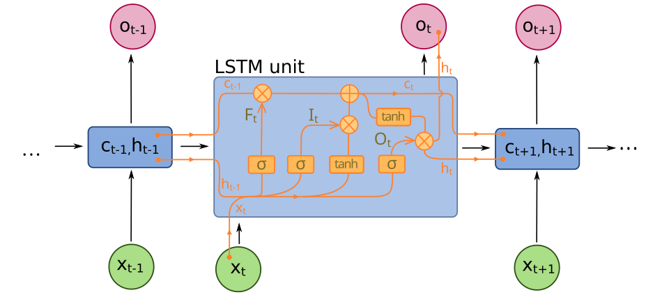Labeled LSTM cell with forget, input, and output gates (Image: fdeloche, CC BY-SA 4.0, via Wikimedia Commons) 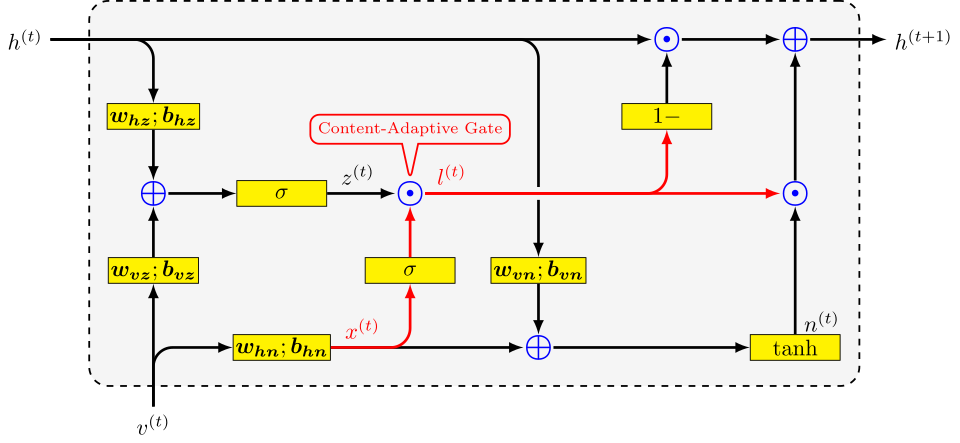GRU cell with update and reset gates (Image: Chankahou0968, CC BY-SA 4.0, via Wikimedia Commons)