Regression in Neural Networks: Linear, Logistic & Model Building

TAKEAWAYS:

• Regression in neural networks maps input data to continuous or discrete outputs using linear/logistic functions, forming the basis for supervised learning.
• Linear regression minimizes squared error via gradient descent, while logistic regression uses sigmoid activation for binary classification.
• Polynomial regression extends linear models by adding non-linear terms (e.g., $x^2$, $x^3$) to fit complex patterns.
• Model evaluation relies on metrics like Mean Squared Error (MSE), Mean Absolute Error (MAE), and R² score.
• Real-world applications include Khalti’s fraud detection (logistic regression), NTC’s network traffic prediction (linear regression), and Daraz’s demand forecasting (polynomial regression).
• Overfitting is mitigated via regularization (L1/L2) and cross-validation.

---

1. Introduction to Regression in Neural Networks

Regression is a supervised learning technique that predicts continuous (regression) or discrete (classification) outputs from input data. In neural networks, regression serves as:

• A single-neuron model (perceptron with linear activation).
• A building block for multi-layer perceptrons (MLPs).
• A baseline for comparing non-linear models (e.g., kernel methods).

Key Types of Regression

---

2. Linear Regression: The Foundation

Linear regression models the relationship between input $x$ and output $y$ as: $$y=w\cdot x+b$$ where:

• $w$ = weight (slope),
• $b$ = bias (intercept).

How It Works: Gradient Descent

The goal is to minimize the Mean Squared Error (MSE): $$\text{MSE}=\frac{1}{n}\sum _{i=1}^n(y_i-{\hat{y}}_i{)}^2$$ Steps:

1. Initialize $w$ and $b$ randomly.
2. Compute gradients: $$\frac{\partial \text{MSE}}{\partial w}=-\frac{2}{n}\sum (x_i(y_i-{\hat{y}}_i))$$ $$\frac{\partial \text{MSE}}{\partial b}=-\frac{2}{n}\sum (y_i-{\hat{y}}_i)$$
3. Update weights: $$w:=w-\alpha \cdot \frac{\partial \text{MSE}}{\partial w},b:=b-\alpha \cdot \frac{\partial \text{MSE}}{\partial b}$$ where $\alpha$ = learning rate.

Worked Example: Predicting NTC’s Network Traffic

Scenario: NTC wants to predict daily internet usage ($y$) based on temperature ($x$) in Kathmandu. Data:

Steps:

1. Plot data (linear trend observed):

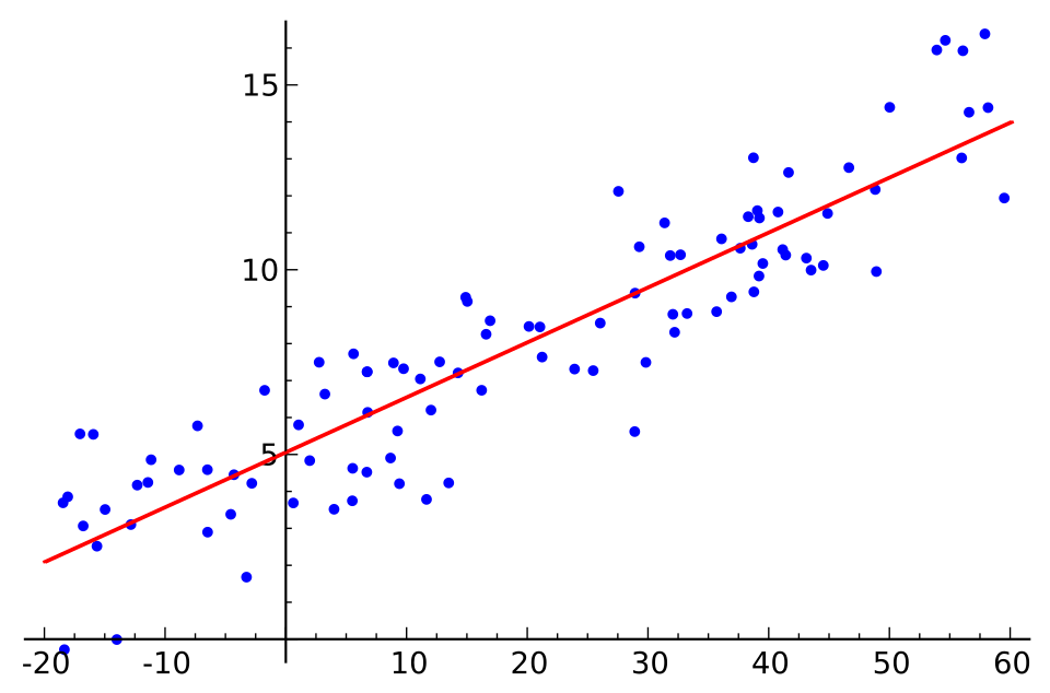Temperature vs. Internet Usage (NTC Data) (Image: Sewaqu, Public domain, via Wikimedia Commons)

*(Imagine a scatter plot with a best-fit line.)*

2. **Initialize:** $w=0.1$, $b=0$, $\alpha =0.01$.
3. **Iteration 1:**
- Predict $\hat{y}=0.1\cdot 10+0=1$ (vs. actual 500).
- Compute gradients and update $w$, $b$.
4. **After 100 iterations:** $w\approx 60$, $b\approx -100$.
- Final model: $y=60x-100$.

**Interpretation:**
- For every 1°C increase, usage rises by **60 GB**.
- **MSE = 12,000** (high error → need more data or polynomial terms).

---

### **3. Logistic Regression: Binary Classification**
Logistic regression predicts **probabilities** (0 to 1) using the **sigmoid function**:
$$\sigma (z)=\frac{1}{1+e^{-z}},z=w\cdot x+b$$
**Output Interpretation:**
- $\sigma (z)<0.5$ → Class 0.
- $\sigma (z)\ge 0.5$ → Class 1.

#### **Loss Function: Cross-Entropy**
$$\text{Loss}=-\frac{1}{n}\sum [y_i\log ({\hat{y}}_i)+(1-y_i)\log (1-{\hat{y}}_i)]$$
**Gradient Descent Update:**
$$w:=w-\alpha \cdot \frac{\partial \text{Loss}}{\partial w},\frac{\partial \text{Loss}}{\partial w}=\frac{1}{n}\sum ({\hat{y}}_i-y_i)x_i$$

#### **Worked Example: Khalti’s Fraud Detection**
**Scenario:** Khalti flags transactions as fraudulent (1) or legitimate (0) based on amount ($x$) and time ($t$).
**Data:**
| Amount (₹) | Time (hrs) | Fraud (1/0) |
|------------|------------|-------------|
| 500        | 14         | 1           |
| 2000       | 9          | 0           |
| 1000       | 16         | 1           |

**Steps:**
1. **Feature Engineering:** Combine $x$ and $t$ into $z=w_1\cdot \text{Amount}+w_2\cdot \text{Time}+b$.
2. **Sigmoid Output:** $\hat{y}=\sigma (z)$.
3. **Train Model:**
- After 50 iterations: $w_1=0.002$, $w_2=0.1$, $b=-3$.
- For ₹500 at 14 hrs: $z=0.002\cdot 500+0.1\cdot 14-3=0.9$ → $\sigma (0.9)=0.71$ → **Flag as fraud (1)**.

**Visualization:**

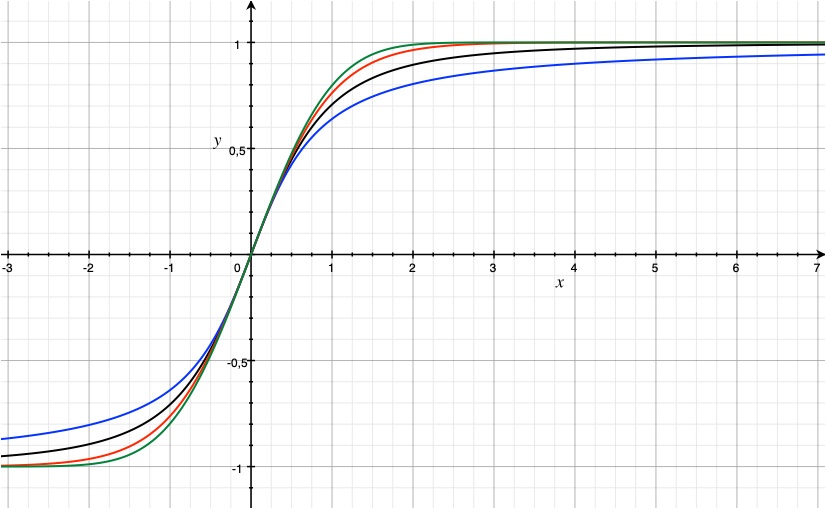Logistic Regression Decision Boundary (Image: Eric.LEWIN, CC BY 4.0, via Wikimedia Commons)

*(Shows how $z$ maps to probability and class labels.)*

---

### **4. Polynomial Regression: Capturing Non-Linearity**
Linear regression fails when data follows **curves**. Polynomial regression adds higher-order terms:
$$y=w_{1}x+w_2{x}^2+w_3{x}^3+\cdots +b$$

#### **Worked Example: Daraz’s Demand Forecasting**
**Scenario:** Daraz observes that product demand ($y$) peaks at moderate prices ($x$) but drops at extremes.
**Data:**
| Price (₹) | Demand (units) |
|-----------|----------------|
| 500       | 100            |
| 1000      | 500            |
| 1500      | 300            |
| 2000      | 50             |

**Steps:**
1. **Add $x^2$ term:**
   $$y=w_{1}x+w_2{x}^2+b$$
2. **Train Model:**
   - After optimization: $y=-0.0005x^2+1.2x-100$.
3. **Plot Fit:**

*(Shows a parabola peaking at ₹1200.)*

**Interpretation:**
- Demand **increases** up to ₹1200, then **decreases** (non-linear effect).

---

### **5. Model Evaluation Metrics**
| **Metric**               | **Formula**                          | **Interpretation**                          |
|--------------------------|--------------------------------------|---------------------------------------------|
| **MSE**                  | $\frac{1}{n}\sum (y_i-{\hat{y}}_i{)}^2$ | Average squared error (lower = better).    |
| **MAE**                  | $\frac{1}{n}\sum |y_i-{\hat{y}}_i|$ | Average absolute error.                     |
| **R² Score**             | $1-\frac{{\text{SS}}_{\text{res}}}{{\text{SS}}_{\text{tot}}}$ | % variance explained (1 = perfect fit).   |

**Example:**
For NTC’s traffic model ($y=60x-100$):
- **MSE = 12,000**, **R² = 0.85** → 85% variance explained.

---

### **6. Overfitting and Regularization**
**Problem:** High-degree polynomials fit training data but fail on test data.
**Solutions:**
1. **L1 Regularization (Lasso):**
$$\text{Loss}=\text{MSE}+\lambda \sum |w_i|$$
(Encourages sparsity; some $w_i=0$.)
2. **L2 Regularization (Ridge):**
$$\text{Loss}=\text{MSE}+\lambda \sum w_i^2$$
(Shrinks weights smoothly.)

**Example:**
For Daraz’s demand model, add **L2 penalty ($\lambda =0.1$)** to prevent overfitting.

---

### **7. Real-World Applications in Nepal**
| **Company/App**  | **Regression Type**       | **Use Case**                                  |
|------------------|---------------------------|-----------------------------------------------|
| **Khalti**       | Logistic Regression      | Fraud detection (binary: fraud/legit).        |
| **NTC**          | Linear Regression        | Predicting network traffic spikes.            |
| **Daraz**        | Polynomial Regression    | Optimizing product pricing.                   |
| **NEPSE**        | Linear Regression        | Stock price trend analysis.                   |
| **Pathao**       | Ridge Regression         | Demand forecasting for driver allocation.    |

---

### **8. Exam Tip: What to Focus On**
1. **Derive the update rules** for linear/logistic regression from scratch (show gradients).
2. **Compare MSE vs. MAE vs. R²** in terms of sensitivity to outliers.
3. **Explain overfitting** with a **polynomial regression plot** (high-degree vs. low-degree).
4. **Link to neural networks:**
- A single neuron with linear activation = linear regression.
- A neuron with sigmoid activation = logistic regression.
5. **Practical question:** Given data, **choose** between linear/logistic/polynomial regression and justify.

---
```mermaid
flowchart LR
 A[Input Data] --> B[Feature Engineering]
 B --> C[Choose Regression Type]
 C -->|Linear| D[Linear Regression\n(MSE Loss)]
 C -->|Binary| E[Logistic Regression\n(Cross-Entropy Loss)]
 C -->|Non-linear| F[Polynomial Regression\n(Add x², x³)]
 D & E & F --> G[Train Model\n(Gradient Descent)]
 G --> H[Evaluate\n(MSE, R², MAE)]
 H -->|Overfit?| I[Apply L1/L2 Regularization]
 I --> J[Final Model]