Data Warehousing and Data MiningUnit 88 min read
Clustering Techniques: Algorithms, Applications & Real-World Use
Unit 8 of Data Warehousing and Data Mining explores unsupervised learning’s clustering techniques—k-means, k-medoids, hierarchical, DBSCAN—with visual algorithms, distance metrics, and real-world examples from eSewa fraud detection to Daraz customer segmentation.
What is Clustering?
Clustering is an unsupervised learning technique that groups similar data points together based on their features, without predefined labels. Unlike supervised classification (e.g., spam detection), clustering discovers hidden patterns in data.
Key Differences: Clustering vs. Classification
| Aspect | Clustering | Classification |
|---|---|---|
| Labels | No labels (unsupervised) | Requires labeled data (supervised) |
| Goal | Find natural groupings | Predict predefined categories |
| Output | Clusters (e.g., "Group A," "Group B") | Class labels (e.g., "Spam," "Not Spam") |
| Example | Customer segmentation in Daraz | Fraud detection in eSewa transactions |
1. Centroid-Based Clustering: K-Means
How K-Means Works
- Initialize: Randomly select k centroids (cluster centers).
- Assign: Assign each data point to the nearest centroid (using Euclidean distance).
- Update: Recalculate centroids as the mean of all points in each cluster.
- Repeat: Until centroids stabilize (convergence).
Euclidean Distance Formula
For two points and :
Worked Example: K-Means (K=2)
Data: (185, 72), (170, 56), (168, 60), (179, 68), (182, 72), (188, 77) Initial Centroids: (185, 72) and (170, 56)
Iteration 1
| Point | Distance to C1 (185,72) | Distance to C2 (170,56) | Cluster |
|---|---|---|---|
| (185,72) | 0 | 15.81 | C1 |
| (170,56) | 15.81 | 0 | C2 |
| (168,60) | 17.32 | 4.47 | C2 |
| (179,68) | 11.40 | 12.20 | C1 |
| (182,72) | 7.07 | 17.03 | C1 |
| (188,77) | 6.40 | 20.62 | C1 |
New Centroids:
- C1: Mean of (185,72), (179,68), (182,72), (188,77) = (183.5, 71.25)
- C2: Mean of (170,56), (168,60) = (169, 58)
Iteration 2
Reassign points to new centroids and repeat until convergence.
K-Means++ for Smarter Initialization
Instead of random centroids, K-Means++ selects initial centroids to maximize distance between them:
- Pick the first centroid uniformly at random.
- Pick the next centroid with probability proportional to its squared distance from existing centroids.
- Repeat until k centroids are chosen.
Example: For points A1(3,11), A2(3,6), A3(9,5), A4(6,9), A6(7,5), A7(2,3), A8(5,10), with A1 as the first centroid:
- Next centroid: A8 (far from A1).
- Third centroid: A3 (far from A1 and A8).
Advantages & Limitations of K-Means
| Advantages | Limitations |
|---|---|
| Fast (O(n·k·i)) | Sensitive to initial centroids |
| Works well for spherical clusters | Requires pre-specifying k |
| Scalable for large datasets | Struggles with non-spherical clusters |
2. K-Medoids (PAM)
Unlike K-Means (which uses means), K-Medoids uses actual data points as centroids (medoids). More robust to outliers.
How K-Medoids Works
- Initialize: Randomly select k medoids.
- Assign: Assign each point to the nearest medoid.
- Swap: For each cluster, find the point that minimizes total distance if swapped with the current medoid.
- Repeat: Until no improvement.
Worked Example: K-Medoids (K=2)
Data: {(70,85), (65,80), (72,88), (75,90), (60,50), (65,60)} Initial Medoids: (70,85) and (60,50)
Iteration 1
| Point | Distance to M1 (70,85) | Distance to M2 (60,50) | Cluster |
|---|---|---|---|
| (70,85) | 0 | 35.36 | M1 |
| (65,80) | 5.83 | 30.00 | M1 |
| (72,88) | 3.61 | 37.42 | M1 |
| (75,90) | 5.39 | 39.05 | M1 |
| (60,50) | 35.36 | 0 | M2 |
| (65,60) | 25.50 | 10.00 | M2 |
Check for Better Medoids:
- For M1’s cluster, test swapping (65,80) or (72,88). Suppose (72,88) reduces total distance → new medoid.
- For M2’s cluster, (65,60) is already the best choice.
3. Hierarchical Clustering
Builds a dendrogram (tree of clusters) either:
- Agglomerative (bottom-up): Start with each point as a cluster, merge the closest pairs.
- Divisive (top-down): Start with one cluster, split recursively.
Example: Agglomerative Clustering
Data: {(2,10), (2,5), (8,4), (5,8), (7,5)} Distance Metric: Euclidean
Step-by-Step Merging
- Merge (2,5) and (7,5) → Cluster C1 (distance = 5).
- Merge (8,4) and (5,8) → Cluster C2 (distance = 4.12).
- Merge C1 and C2 → Final cluster.
graph TD
    A[(2,10)] --> B[{(2,5), (7,5)}]
    C[(8,4)] --> D[{(5,8)}]
    B --> E[{(2,5), (7,5), (8,4), (5,8), (2,10)}]
    D --> E
4. DBSCAN (Density-Based Clustering)
Groups points based on density (no need to specify k).
- Parameters:
- ε (eps): Maximum distance between two points to be considered neighbors.
- minPts: Minimum points to form a dense region (core point).
- Outliers: Points not in any cluster.
How DBSCAN Works
- Find a core point (with ≥ minPts neighbors within ε).
- Expand the cluster by including all density-reachable points.
- Repeat for remaining points.
Example:
- ε = 5, minPts = 3
- Points: (1,2), (2,3), (3,4), (10,11), (11,12), (12,13)
- Cluster 1: {(1,2), (2,3), (3,4)}
- Cluster 2: {(10,11), (11,12), (12,13)}
- Outlier: None (if all points are dense).
## In the Real World
eSewa Fraud Detection
- Idea: DBSCAN clusters unusual transaction patterns (e.g., rapid small payments).
- How: Points with low density (e.g., 100 transactions in 1 hour) flag potential fraud.
Daraz Customer Segmentation
- Idea: K-Means groups customers by purchase history (e.g., "High-Spenders," "Bargain Hunters").
- How: Centroids represent average spending/preferences per cluster.
NTC Network Traffic Analysis
- Idea: Hierarchical clustering identifies peak usage regions (e.g., Kathmandu vs. Pokhara).
- How: Agglomerative clustering merges similar time slots into "busy periods."
Khalti Loan Risk Assessment
- Idea: K-Medoids clusters borrowers by credit risk (medoids = "typical" high/low-risk profiles).
- How: Outliers (e.g., sudden large loans) trigger manual review.
## Visualizing Clustering Algorithms
1. K-Means Convergence (Game Tree)
graph TD
    A["Initial Centroids: C1, C2"] --> B["Assign Points"]
    B --> C["Update Centroids"]
    C --> D{"Converged?"}
    D -->|"No"| B
    D -->|"Yes"| E["Final Clusters"]
2. DBSCAN Density Regions
graph TD
    A["Core Point"] --> B["Neighbors within ε"]
    B --> C["Expand Cluster"]
    D["Border Point"] --> E["Assigned to Cluster"]
    F["Noise"] --> G["Outlier"]
3. Hierarchical Dendrogram
graph TD
    A[(2,10)] --> B["Cluster 1"]
    C[(2,5)] --> B
    D[(8,4)] --> E["Cluster 2"]
    F[(5,8)] --> E
    B --> G["Final Cluster"]
    E --> G
## Exam Tip
For K-Means/K-Medoids:
- Always show distance calculations and centroid/medoid updates step-by-step.
- Use Euclidean distance formula explicitly in answers.
- If initial centroids aren’t given, assume first k points or K-Means++.
For Hierarchical Clustering:
- Draw the dendrogram and label merge steps.
- Specify whether it’s agglomerative or divisive.
For DBSCAN:
- Define ε and minPts clearly.
- Identify core points, border points, and noise.
Comparisons:
- K-Means vs. K-Medoids: Centroids (mean) vs. medoids (actual points).
- Hierarchical vs. K-Means: Tree structure vs. flat clusters; no k needed vs. k required.
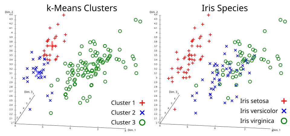 Example of K-Means grouping 2D points into 3 clusters (Image: Chire, Public domain, via Wikimedia Commons)
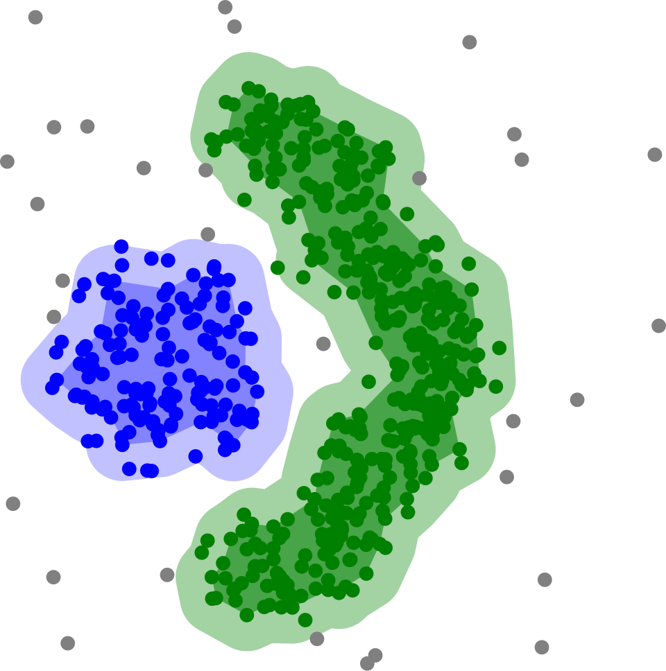 DBSCAN identifying dense regions in a scatter plot (Image: Chire, CC BY-SA 3.0, via Wikimedia Commons)
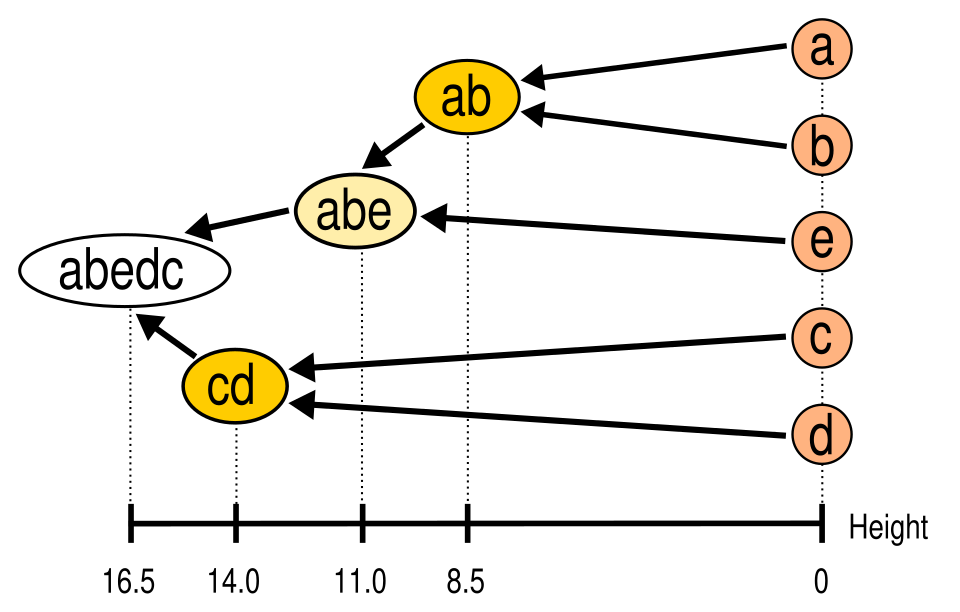 Agglomerative clustering tree for 6 data points (Image: This picture is a work by Emmanuel Douzery. Please credit th, CC BY-SA 4.0, via Wikimedia Commons)
Based on the TU BSc CSIT syllabus for Data Warehousing and Data Mining (CSC410), unit 8.
Discussion
Loading…