Data Warehousing and Data MiningUnit 412 min read
Data Cube, OLAP & Multidimensional Analysis: OLAP Operations, Cube Design, Drill-Down
Unit 4 of Data Warehousing and Data Mining covers OLAP (Online Analytical Processing) architectures, data cube structures, OLAP operations (slice, dice, roll-up, drill-down), and their implementation in data warehouses. Learn how to design star/snowflake schemas, compute aggregations, and optimize queries for business
TAKEAWAYS:
- Data cubes are multidimensional arrays (e.g.,
Time × Product × Region × Sales) that enable fast OLAP queries by precomputing aggregations. - OLAP operations (slice, dice, roll-up, drill-down, pivot) let analysts explore data without rewriting SQL—critical for dashboards.
- Star schemas (fact tables + dimension tables) are simpler than snowflakes but may suffer from redundancy; snowflakes normalize dimensions at the cost of query complexity.
- Aggregation levels (e.g., daily → monthly → yearly) trade storage space for query speed—choose based on query patterns.
- Materialized views (precomputed cubes) speed up OLAP but increase storage and refresh costs.
- Drill-through connects OLAP results to transactional data for deeper investigation (e.g., "Why did sales drop in Region X?").
1. Data Warehousing vs. OLTP: Why OLAP?
Data warehouses store historical, integrated, and summarized data for analytical processing, unlike OLTP systems (e.g., bank transactions) that handle real-time, detailed operations.
flowchart LR
    A["OLTP Systems"] -->|"Fast,<br>Transactional"| B["Bank ATM<br>eSewa Payment<br>Pathao Order"]
    C["OLAP Systems"] -->|"Slow,<br>Analytical"| D["Sales Dashboard<br>NTC Traffic Analysis<br>NEPSE Stock Trends"]
    A -->|"Example"| E["INSERT, UPDATE, DELETE"]
C -->|"Example"| F["SUM(sales), AVG(price), GROUP BY region"]| OLTP | OLAP |
|---|---|
| Normalized tables | Denormalized (star/snowflake) |
| Short transactions (<2 sec) | Complex queries (minutes) |
| Example: Khalti payment | Example: Daraz sales report |
2. The Data Cube: Multidimensional Data Model
A data cube is a generalization of a 2D pivot table to N dimensions (e.g., Time × Product × Region × Sales). Each dimension has hierarchies (e.g., Year → Quarter → Month).
How Cubes Work
- Cells store aggregated values (e.g.,
SUM(sales)). - Dimensions define axes (e.g.,
Product,Date,Store). - Measures are the values being aggregated (e.g.,
Revenue,Quantity).
Example: Sales Data Cube
Product: Laptop, Mobile, TV
Time:   2023-Q1, 2023-Q2
Region: Kathmandu, Pokhara, Lalitpur
Measure: Sales ($)
Visualization:
graph TD
    A["Product"] --> B["Laptop"]
    A --> C["Mobile"]
    A --> D["TV"]
    E["Time"] --> F["2023-Q1"]
    E --> G["2023-Q2"]
    H["Region"] --> I["Kathmandu"]
    H --> J["Pokhara"]
    H --> K["Lalitpur"]
    B -->|"Sales"| L["1000"]
    C -->|"Sales"| M["1500"]
    D -->|"Sales"| N["800"]
Cube Operations
| Operation | Definition | Example |
|---|---|---|
| Slice | Fix one dimension, show the rest. | Fix Region = Kathmandu, show Product × Time × Sales. |
| Dice | Select a sub-cube by constraints on multiple dimensions. | Show Product = Laptop AND Time = 2023-Q1. |
| Roll-Up | Aggregate data up the hierarchy (drill-up). | Roll-up Month → Quarter for total Q1 sales. |
| Drill-Down | Move down the hierarchy (more detail). | Drill-down Region → District to see sales by ward. |
| Pivot | Rotate dimensions (e.g., swap Product and Time axes). |
Swap axes to compare Sales by Time vs. Sales by Product. |
| Drill-Through | Link OLAP result to transactional data (e.g., click a sales cell to see orders). | Click "Laptop sales in Kathmandu" → see list of orders. |
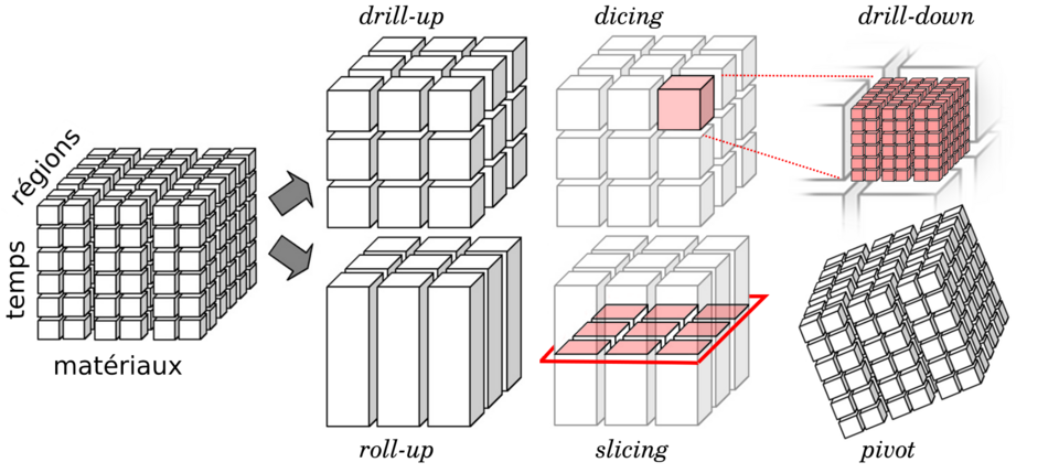 OLAP cube operations diagram (Image: Mquantin, CC BY-SA 4.0, via Wikimedia Commons)
3. Star Schema vs. Snowflake Schema
Both organize data for OLAP but differ in normalization.
Star Schema
- 1 fact table connected directly to dimension tables.
- Pros: Faster queries, simpler joins.
- Cons: Redundancy in dimension tables.
erDiagram
    FACT_SALES ||--o{ DIM_PRODUCT : "1:N"
    FACT_SALES ||--o{ DIM_TIME : "1:N"
    FACT_SALES ||--o{ DIM_REGION : "1:N"
    DIM_PRODUCT {
        int product_id PK
        varchar product_name
        float price
    }
    DIM_TIME {
        int time_id PK
        date sale_date
        varchar quarter
    }
    DIM_REGION {
        int region_id PK
        varchar city
        varchar district
    }
    FACT_SALES {
        int sale_id PK
        int product_id FK
        int time_id FK
        int region_id FK
        int quantity
        float revenue
    }
Snowflake Schema
- Normalized dimension tables (e.g.,
Regionsplits intoCountry,City). - Pros: Less redundancy, smaller tables.
- Cons: More joins → slower queries.
erDiagram
    FACT_SALES ||--o{ DIM_PRODUCT : "1:N"
    FACT_SALES ||--o{ DIM_TIME : "1:N"
    FACT_SALES ||--o{ DIM_CITY : "1:N"
    DIM_CITY ||--|| DIM_COUNTRY : "1:N"
    DIM_PRODUCT { int product_id PK }
    DIM_TIME { int time_id PK }
    DIM_CITY { int city_id PK }
    DIM_COUNTRY { int country_id PK }
When to Use Which?
| Schema | Use Case | Example |
|---|---|---|
| Star | Fast queries, simple models | eSewa transaction dashboard |
| Snowflake | Highly normalized data, complex hierarchies | NTC traffic analysis by district |
4. OLAP Operations in Action: Worked Example
Scenario: Daraz wants to analyze sales data for Laptops in Kathmandu for Q1 2023.
Step 1: Define the Cube
Dimensions:
Product(Laptop, Mobile, TV)Time(2023-Q1, 2023-Q2)Region(Kathmandu, Pokhara, Lalitpur)
Measures:
Quantity SoldRevenue ($)
Step 2: Apply OLAP Operations
- Slice: Fix
Region = Kathmandu.- Result:
Product × Time × Quantityfor Kathmandu only.
- Result:
- Dice: Add
Product = Laptop.- Result: Only Laptop sales in Kathmandu for Q1-Q2.
- Drill-Down: Break
TimefromQuartertoMonth.- Now see sales by month (Jan, Feb, Mar).
- Roll-Up: Aggregate
MonthtoQuarter.- Total Q1 sales for Laptops in Kathmandu.
Visual Trace:
graph TD
    A["Full Cube"] --> B["Slice: Region=Kathmandu"]
    B --> C["Dice: Product=Laptop"]
    C --> D["Drill-Down: Time→Month"]
    D --> E["Roll-Up: Month→Quarter"]
SQL Equivalent
-- Slice + Dice (Region=Kathmandu, Product=Laptop)
SELECT Time, SUM(Quantity) as TotalSold
FROM FactSales
JOIN DimProduct ON FactSales.product_id = DimProduct.product_id
JOIN DimRegion ON FactSales.region_id = DimRegion.region_id
WHERE DimRegion.city = 'Kathmandu'
  AND DimProduct.product_name = 'Laptop'
GROUP BY Time;

-- Drill-Down (Month-level detail)
SELECT Month, SUM(Quantity)
FROM FactSales
JOIN DimTime ON FactSales.time_id = DimTime.time_id
WHERE DimTime.quarter = 'Q1'
GROUP BY Month;
5. Materialized Views and Pre-Aggregation
OLAP cubes are often precomputed (materialized) to speed up queries.
Trade-offs
| Approach | Pros | Cons | Example |
|---|---|---|---|
| On-the-fly aggregation | Always up-to-date | Slow for complex queries | Google Analytics (real-time) |
| Materialized cube | Fast queries | Storage cost, stale data | NEPSE stock trend dashboards |
Example: NEPSE Stock Analysis
- Cube:
Stock × Date × Sector × Volume. - Precompute: Daily, weekly, and monthly aggregates.
- Query: "Show NEPSE volume trends by sector for 2023."
- If precomputed: <1 sec.
- If computed on-the-fly: >10 sec.
6. Real-World Applications
1. eSewa: Fraud Detection via OLAP
- Cube:
User × Transaction × Time × Amount × Location. - Operation: Drill-down on suspicious transactions (e.g.,
Amount > $500inKathmandu). - Outcome: Detects unusual patterns (e.g., multiple high-value transactions from one IP).
2. Daraz: Inventory Optimization
- Cube:
Product × Region × Time × Sales × Stock. - Operation: Roll-up sales by region to identify slow-moving items.
- Outcome: Adjusts stock levels dynamically (e.g., reduce TV stock in Pokhara if sales are low).
3. NTC: Traffic Flow Analysis
- Cube:
Road × Time × VehicleType × CongestionLevel. - Operation: Slice by
Road = Ring Road+ Drill-down toHourlydata. - Outcome: Identifies peak congestion hours to optimize traffic signals.
4. NEPSE: Investor Trends
- Cube:
Stock × InvestorType × Time × Volume. - Operation: Pivot to compare
Institutionalvs.Retailinvestor activity. - Outcome: Helps traders spot market sentiment shifts.
5. Pathao: Driver Performance
- Cube:
Driver × Route × Time × Rating × Earnings. - Operation: Dice for
Rating < 3.5+ Drill-through to trip logs. - Outcome: Flags poor-performing drivers for training.
7. Exam Tip: How to Score Full Marks
Define Clearly:
- Start every answer with definitions (e.g., "A data cube is a multidimensional structure that stores aggregated data along dimensions like Time, Product, and Region.").
- Example:
"OLAP operations are actions performed on a data cube to analyze data without altering the underlying schema. The six primary operations are slice, dice, drill-down, roll-up, pivot, and drill-through."
Use Diagrams:
- Draw star/snowflake schemas for schema questions.
- Show cube operations with arrows (e.g., slice → dice → drill-down).
- Example:
Original Cube (3D) → [Slice] → 2D Table → [Dice] → Sub-Table
Relate to Real Systems:
- Tie examples to Nepali apps (eSewa, Daraz, NTC) or global tools (Google Analytics, Power BI).
- Example:
"In Daraz’s OLAP system, a ‘dice’ operation could isolate laptop sales in Kathmandu for Q1 to identify best-selling models."
Avoid Common Mistakes:
- ❌ "Roll-up and drill-down are the same." → Wrong! Roll-up aggregates up (e.g., month → quarter), drill-down goes down (e.g., region → district).
- ❌ "Star schema is normalized." → Wrong! It’s denormalized for speed.
- ❌ "Materialized views are always better." → Context matters! Mention trade-offs (storage vs. speed).
Practice SQL-OLAP Mapping:
- Convert OLAP operations to SQL. Example:
OLAP Operation SQL Equivalent Slice WHERE dimension = 'value'Dice WHERE dim1 = 'val1' AND dim2 = 'val2'Roll-Up GROUP BY higher_level_dimension
- Convert OLAP operations to SQL. Example:
For Numerical Questions:
- Show every step of calculations (e.g., aggregating sales by region).
- Example:
"Given sales data for Laptops in Kathmandu: Jan=100, Feb=150, Mar=120. Roll-up to quarter: Q1 Total = 100 + 150 + 120 = 370."
8. Quick Revision Table
| Concept | Key Idea | Example |
|---|---|---|
| Data Cube | N-dimensional array for OLAP. | Time × Product × Region × Sales |
| Star Schema | Fact table + denormalized dimensions. | eSewa transaction dashboard |
| Snowflake | Normalized dimensions (more joins). | NTC traffic analysis by district |
| Slice | Fix one dimension. | Show Product × Time for Region=KTM. |
| Dice | Filter multiple dimensions. | Show Laptop AND Q1 AND Kathmandu. |
| Drill-Down | Add detail (e.g., month → day). | Break Quarter into Month. |
| Roll-Up | Aggregate up (e.g., day → month). | Sum Daily Sales to Monthly. |
| Pivot | Rotate axes (e.g., swap Product and Time). |
Compare Sales by Time vs. by Product. |
| Materialized View | Precomputed cube for speed. | NEPSE stock trend dashboards. |
Based on the TU BSc CSIT syllabus for Data Warehousing and Data Mining (CSC410), unit 4.
Discussion
Loading…