EconomicsUnit 510 min read
Income, Employment & Keynesian Theory: Circular Flow, AD-AS, Multiplier
Unit 5 of Economics explains how national income is determined, how employment is created, and why economies face unemployment—using Keynesian models like circular flow, aggregate demand-supply, and the multiplier effect.
TAKEAWAYS:
- Circular flow shows how money moves between households and firms, creating income and spending.
- Aggregate demand (AD) is total spending by households, firms, government, and foreign buyers.
- Aggregate supply (AS) is total output firms produce at different price levels—short-run vs. long-run curves differ.
- Equilibrium income is where AD = AS; shifts in AD cause changes in employment and output.
- Multiplier effect explains how an initial spending boost creates more income through repeated spending cycles.
- Unemployment types (frictional, structural, cyclical) arise when AD is too low for full employment.
1. Circular Flow of Income
The economy is like a circular system where money and goods/services keep moving between households and firms.
flowchart TD
    A["Households"] -->|"Factors of Production (Land, Labour, Capital, Entrepreneurship)"| B["Firms"]
    B -->|"Goods & Services"| A
    A -->|"Consumption Expenditure (C)"| B
    B -->|"Wages, Rent, Interest, Profit"| A
    C["Government"] -->|"Taxes"| A
    C -->|"Government Spending (G)"| B
    D["Foreign Sector"] -->|"Exports (X)"| B
    D -->|"Imports (M)"| A
Key Points:
- Households supply factors of production (land, labour, capital, entrepreneurship) to firms.
- Firms pay income (wages, rent, interest, profit) to households.
- Households spend on goods/services (consumption, C).
- Government collects taxes (T) and spends (G).
- Foreign sector buys exports (X) and sells imports (M).
Why is this important?
- Shows how income is earned and spent, keeping the economy running.
- If spending (AD) falls, firms produce less → unemployment rises.
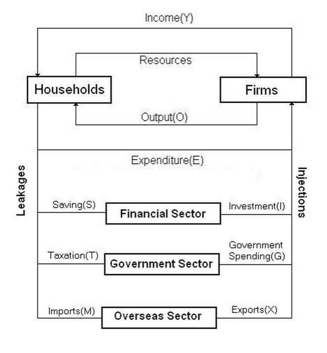 Households, firms, government, and foreign sector interactions (Image: Ari89, CC0, via Wikimedia Commons)
2. Aggregate Demand (AD) and Its Components
AD = Total demand for goods/services in an economy at different price levels. It is made up of:
- Consumption (C) – Spending by households.
- Investment (I) – Spending by firms on machinery, buildings, etc.
- Government Spending (G) – Roads, schools, hospitals.
- Net Exports (X – M) – Exports minus imports.
AD Curve Shape:
- Downward-sloping because:
- Wealth effect: Lower prices → people feel richer → spend more.
- Interest rate effect: Lower prices → banks lend more → investment rises.
- Exchange rate effect: Lower domestic prices → exports rise, imports fall.
Graph of AD:
graph LR
    A["Price Level (P)"] -->|"↓"| B["AD"]
    B -->|"↑"| C["Real GDP (Y)"]
Example: If the price level falls from 120 to 100, AD increases from ₹500 crore to ₹600 crore (due to higher consumption and investment).
3. Aggregate Supply (AS) – Short-Run vs. Long-Run
AS = Total output firms are willing to produce at different price levels.
Short-Run AS (SRAS)
- Upward-sloping because:
- Firms increase production if prices rise (higher profits).
- Fixed factors (like machinery) cannot be changed immediately.
- Assumption: Some resources are unused (unemployment exists).
Long-Run AS (LRAS)
- Vertical at full employment (Yf) because:
- All resources are fully employed.
- No unused capacity—economy operates at potential GDP.
- Price changes do not affect output in the long run.
Graph of AS:
graph LR
    A["Price Level (P)"] -->|"↑"| B["SRAS"]
    B -->|"↑"| C["Real GDP (Y)"]
    D["LRAS"] -->|"Vertical"| E["Full Employment (Yf)"]
Why the difference?
- Short-run: Firms can hire more workers, use idle machines.
- Long-run: Economy hits its maximum capacity—no more growth possible without new technology or resources.
4. Equilibrium Income (AD = AS)
Equilibrium occurs where AD = AS.
- At this point:
- Planned spending = Actual output.
- No unsold goods (inventories stable).
- Full employment (if at LRAS).
Graph of Equilibrium:
graph LR
    A["AD"] -->|"Intersects"| B["SRAS"]
    B -->|"Equilibrium"| C["Y* (Equilibrium Output)"]
    D["LRAS"] -->|"Vertical"| C
Example: If AD = ₹1000 crore and AS = ₹1000 crore, the economy is in equilibrium at Y = ₹1000 crore.
What if AD shifts?
| Shift in AD | Effect on Output (Y) | Effect on Employment | Effect on Price Level |
|---|---|---|---|
| AD ↑ (Right shift) | Y ↑ | Employment ↑ | P ↑ (Short-run) |
| AD ↓ (Left shift) | Y ↓ | Unemployment ↑ | P ↓ (Short-run) |
Why does this matter?
- If AD is too low, firms produce less → unemployment rises (recession).
- If AD is too high, prices rise → inflation.
5. The Multiplier Effect
When government or firms spend more, income increases more than the initial spending due to the multiplier effect.
How it works:
- Initial spending (ΔI or ΔG) → Firms produce more → Income rises by ΔI.
- Households spend part of new income (MPC) → Firms get more orders → Income rises again.
- This keeps happening until total income increase = Initial spending × Multiplier (k).
Formula: Where:
- MPC (Marginal Propensity to Consume) = Fraction of extra income spent.
- MPS (Marginal Propensity to Save) = Fraction of extra income saved.
Example: If MPC = 0.8, then:
- If government spends ₹100 crore, total income rises by:
Why is this useful?
- Shows how small changes in investment or government spending can boost the economy.
- Helps explain why recessions are deep (small spending cuts → big income drops).
6. Types of Unemployment (Why AD Matters)
When AD is too low, firms cut production → unemployment rises.
| Type | Cause | Example in Nepal |
|---|---|---|
| Frictional | Workers moving between jobs | A teacher quits to find a better school |
| Structural | Skills mismatch or tech changes | Factory workers replaced by machines |
| Cyclical | Low AD (recession) | Many workers laid off during COVID-19 |
How AD affects unemployment:
- If AD falls, firms reduce hiring → cyclical unemployment rises.
- If AD rises, firms hire more → unemployment falls.
7. Policy Implications (Fiscal Policy)
Governments can shift AD to fix unemployment or inflation.
| Problem | Policy | Effect on AD | Example |
|---|---|---|---|
| High Unemployment | Increase G or cut T | AD shifts right | Nepal builds more roads → more jobs |
| High Inflation | Decrease G or raise T | AD shifts left | Government reduces subsidies → less spending |
Example (Nepal):
- 2020 Lockdown: AD fell → unemployment rose → government gave cash aid to poor families (↑C) to boost AD.
Exam Tip: How to Score Full Marks
✅ Understand AD-AS shifts – Always ask:
- Who is spending more/less?
- Is it short-run or long-run?
- Does it affect output or just prices?
✅ Multiplier questions – Remember:
- k = 1 / (1 – MPC)
- Always show calculations (NEB loves step-by-step).
✅ Unemployment types – Link them to AD:
- Cyclical unemployment = Low AD problem.
✅ Real-world examples – Nepal’s economy:
- Remittances (X) boost AD.
- Droughts reduce agricultural output (AS shift left).
✅ Diagrams are key! – Always draw:
- AD-AS equilibrium (label shifts).
- Circular flow (for income explanation).
- Multiplier effect (show repeated spending rounds).
NEB Board-Style Questions (Practice)
Short Answer (5 marks)
"Explain the components of Aggregate Demand with an example from Nepal’s economy." Answer:
- C (Consumption): Nepali families spending on food, clothes.
- I (Investment): A factory buying new machines.
- G (Government): Building a new hospital in Kathmandu.
- X – M (Net Exports): Selling jute to India (X) vs. buying petroleum (M).
"Why is the Short-Run AS curve upward-sloping?" Answer:
- Firms can hire more workers or use idle machinery.
- Higher prices → higher profits → more production.
- But in the long run, all resources are fully used → LRAS is vertical.
Long Answer (10 marks)
"Using AD-AS diagram, explain how an increase in government spending affects equilibrium income and employment. What happens if this spending leads to inflation?" Answer:
- Step 1: Draw initial AD and AS, mark equilibrium at Y1, P1.
- Step 2: Government spends more (G ↑) → AD shifts right to AD’.
- Step 3: New equilibrium at Y2 > Y1 (↑output), P2 > P1 (↑prices).
- Step 4: If Y2 = Full Employment (Yf), further AD increase causes only price rise (inflation).
"Calculate the multiplier effect if MPC = 0.75 and initial investment increases by ₹200 crore." Answer:
- MPC = 0.75 → MPS = 1 – 0.75 = 0.25
- k = 1 / (1 – 0.75) = 4
- Total income increase = 4 × ₹200 crore = ₹800 crore
Common Mistakes to Avoid
❌ Forgetting to label axes in AD-AS diagrams (NEB deducts marks!). ❌ Mixing short-run and long-run AS – Always specify which one you’re using. ❌ Ignoring real-world examples – Nepal’s remittances, droughts, or government policies are highly scored. ❌ Wrong multiplier formula – Always use k = 1 / (1 – MPC).
Final Tip:
- AD shifts = Spending changes (C, I, G, X-M).
- AS shifts = Supply shocks (droughts, oil price changes).
- Multiplier = How spending ripples through the economy.
Good luck! 🚀 Study these diagrams and examples well—they appear every year in NEB exams.
Based on the NEB +2 Humanities syllabus for Economics (Eco), unit 5.
Discussion
Loading…