EconomicsUnit 810 min read
Cost & Revenue: Types, Relationships & Decision-Making
Unit 8 of Economics explores how businesses calculate costs (fixed, variable, total) and revenue (total, average, marginal), their relationships, and how firms use them to make production and pricing decisions—essential for NEB exams.
TAKEAWAYS:
- Costs are classified into fixed (rent, salaries), variable (raw materials, wages), and total (fixed + variable), and their per-unit forms (average and marginal) help firms optimize production.
- Revenue is measured as total revenue (TR), average revenue (AR), and marginal revenue (MR), with key relationships like MR = ΔTR/ΔQ and AR = TR/Q.
- The law of variable proportions explains how marginal product changes as variable inputs (e.g., labor) are added to fixed inputs (e.g., land).
- Firms maximize profit where MR = MC (marginal revenue equals marginal cost), and shutdown rule applies if P < AVC (price < average variable cost).
- Break-even point occurs where TR = TC (total revenue equals total cost), and firms earn normal profit (zero economic profit).
- Revenue and cost curves (TR, AR, MR, TC, AFC, AVC, MC) are visualized to show decision-making rules under different market structures.
1. Introduction to Costs
Costs are the expenses a business incurs to produce goods or services. They can be classified into three main types:
1.1 Fixed Costs (FC)
- Costs that do not change with the level of production in the short run.
- Examples: Rent, insurance, salaries of permanent staff, interest on loans.
- Graphical Representation:
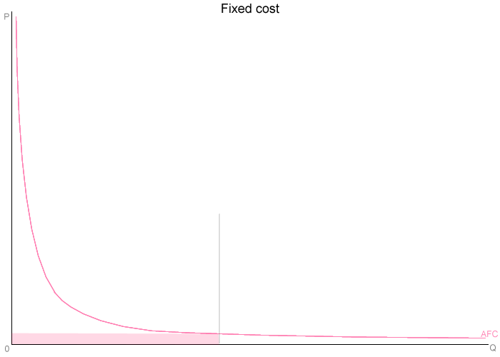 A horizontal line parallel to the x-axis (quantity) showing constant FC regardless of output. (Image: The original uploader was Yunzhong Hou at English Wikibooks., CC BY-SA 2.0, via Wikimedia Commons)
1.2 Variable Costs (VC)
- Costs that change with the level of production.
- Examples: Raw materials, wages of temporary workers, electricity bills.
- Graphical Representation:
1.3 Total Cost (TC)
- Sum of fixed costs (FC) and variable costs (VC).
- Graphical Representation:
2. Per-Unit Costs: Average and Marginal
2.1 Average Fixed Cost (AFC)
- Fixed cost per unit of output.
- Graphical Representation:
2.2 Average Variable Cost (AVC)
- Variable cost per unit of output.
- Graphical Representation:
2.3 Average Total Cost (ATC)
- Total cost per unit of output.
- Graphical Representation:
 A U-shaped curve that lies above the AVC curve by the amount of AFC. (Image: Jarry1250, CC BY-SA 3.0, via Wikimedia Commons)
2.4 Marginal Cost (MC)
- The additional cost of producing one more unit of output.
- Graphical Representation:
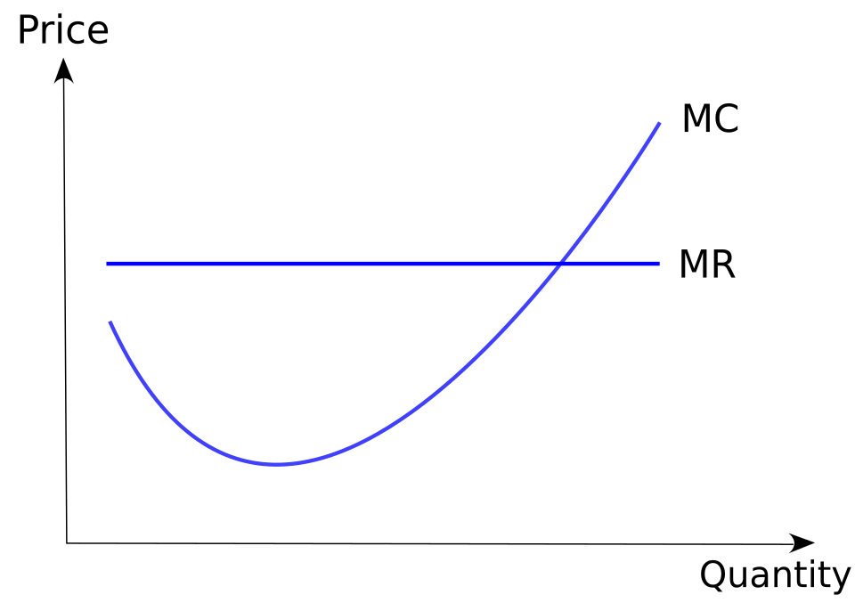 A curve that cuts the AVC and ATC curves at their minimum points. (Image: Jarry1250, CC BY-SA 3.0, via Wikimedia Commons)
3. The Law of Variable Proportions (Returns to a Factor)
This law explains how marginal product changes when one variable input (e.g., labor) is increased while keeping other inputs (e.g., land, capital) fixed.
Stages of Production
Stage I: Increasing Returns
- Marginal Product (MP) increases as more labor is added.
- Example: Adding workers to a fixed plot of land increases output per worker.
Stage II: Diminishing Returns
- MP decreases but remains positive.
- Example: Overcrowding workers on the same land reduces efficiency.
Stage III: Negative Returns
- MP becomes negative (total product decreases).
- Example: Too many workers get in each other’s way, reducing output.
Graphical Representation
Example:
| Labor (L) | Total Product (TP) | Marginal Product (MP) | Stage |
|---|---|---|---|
| 0 | 0 | - | - |
| 1 | 10 | 10 | Stage I |
| 2 | 25 | 15 | Stage I |
| 3 | 40 | 15 | Stage I |
| 4 | 50 | 10 | Stage II |
| 5 | 55 | 5 | Stage II |
| 6 | 55 | 0 | Stage III |
| 7 | 50 | -5 | Stage III |
4. Revenue Concepts
Revenue is the total income a firm earns from selling goods or services.
4.1 Total Revenue (TR)
- Total money received from selling a quantity of goods.
Where:
- = Price per unit
- = Quantity sold
4.2 Average Revenue (AR)
- Revenue per unit sold.
- In perfect competition, .
- In monopoly, .
4.3 Marginal Revenue (MR)
- Additional revenue from selling one more unit.
- Graphical Representation:
5. Relationship Between Cost and Revenue
Firms use cost and revenue curves to make profit-maximizing decisions.
Profit Maximization Rule
A firm maximizes profit where:
- If , the firm should increase output.
- If , the firm should decrease output.
Shutdown Rule
A firm should shut down in the short run if:
- The firm cannot cover its variable costs, so it’s better to stop production temporarily.
Break-Even Point
Occurs where:
- At this point, the firm earns normal profit (zero economic profit).
6. Cost and Revenue in Different Market Structures
| Feature | Perfect Competition | Monopoly |
|---|---|---|
| Number of Firms | Many | One |
| Price Control | Price taker () | Price maker () |
| Profit Maximization | (if ) | |
| Efficiency | Productive & allocative efficiency | Deadweight loss (inefficiency) |
| Example | Agriculture (wheat farming) | Electricity supply (Nepal Electricity Authority) |
7. Solved Examples
Example 1: Calculating Costs
A firm has:
- Fixed Cost (FC) = Rs. 50,000
- Variable Cost (VC) at 5 units = Rs. 20,000
- Variable Cost (VC) at 10 units = Rs. 40,000
Calculate:
- Total Cost (TC) at 10 units.
- Average Variable Cost (AVC) at 10 units.
- Marginal Cost (MC) between 5 and 10 units.
Solution:
Example 2: Profit Maximization
A firm’s demand and cost data:
| Quantity (Q) | Price (P) | TR | MC |
|---|---|---|---|
| 1 | 10 | 10 | 4 |
| 2 | 9 | 18 | 6 |
| 3 | 8 | 24 | 8 |
| 4 | 7 | 28 | 12 |
Find the profit-maximizing quantity and profit.
Solution:
- Calculate :
- between Q=1 and Q=2:
- between Q=2 and Q=3:
- between Q=3 and Q=4:
- Compare and :
- At Q=3, → Profit-maximizing quantity.
- Profit = :
- at Q=3 = Rs. 24
- at Q=3 = (assuming FC=0 for simplicity)
- Profit = Rs. 6
8. NEB Board-Style Questions
Short Answer Questions (SAQ)
- Define marginal cost. Why does the MC curve cut the AVC and ATC curves at their minimum points?
- Explain the law of variable proportions with an example.
- What is the shutdown rule? When should a firm shut down in the short run?
- Distinguish between average revenue and marginal revenue with a diagram.
- Why is the marginal revenue curve below the average revenue curve in a monopoly?
Long Answer Questions (LAQ)
Explain the relationship between total cost, average cost, and marginal cost with the help of a cost schedule and diagram. How does this relationship help a firm in decision-making?
A firm’s total cost and total revenue at different levels of output are given below. Determine:
- The profit-maximizing output.
- The maximum profit.
- Whether the firm should shut down in the short run.
Output (Q) TC TR 1 50 60 2 80 100 3 120 120 4 170 130 "A firm maximizes profit where MR = MC." Explain this statement with the help of a diagram. What happens if the firm produces more or less than this quantity?
Exam Tip
Memorize Key Formulas:
Understand Graphs:
- Draw and label U-shaped ATC, AVC, and MC curves.
- Show profit maximization (MR=MC) and shutdown point (P=AVC).
Apply Concepts to Real Life:
- Example: If a tea shop increases workers but output falls, it’s in Stage III of production.
- Example: If a mobile company reduces prices to sell more phones, it’s following MR=MC rule.
Common Mistakes to Avoid:
- Confusing short-run (fixed costs) and long-run (all costs variable).
- Forgetting that MC cuts AVC and ATC at their minimum.
- Ignoring the shutdown rule ().
NEB Exam Pattern:
- SAQs: Focus on definitions, differences, and short explanations.
- LAQs: Require diagrams, calculations, and real-world applications.
- Numerical Problems: Always show step-by-step calculations.
Final Note: Cost and revenue analysis is the backbone of business decisions. Mastering this unit will help you understand how firms decide what to produce, how much to produce, and at what price—key concepts for both NEB exams and real-world economics! 🚀
Based on the NEB +2 Management syllabus for Economics (Eco), unit 8.
Discussion
Loading…