Business Mathematics IIUnit 913 min read
Simplex Method: Solving Linear Programming Problems
Unit 9 of Business Mathematics II covers the Simplex Method, a systematic algebraic technique for solving linear programming problems with multiple constraints. Learn how to convert constraints into standard form, construct initial and final simplex tables, and interpret optimal solutions for business decisions like co
TAKEAWAYS:
- The Simplex Method solves linear programming problems by moving along the feasible region’s boundary to find the optimal solution.
- Standard form requires all constraints to be equalities (≤ or ≥ converted to =) with slack/surplus variables and a non-negative objective function.
- Simplex tables organize coefficients to iteratively improve the objective function until optimality is reached (no negative coefficients in the bottom row).
- Pivoting selects the entering and leaving variables based on the minimum ratio test and most negative coefficient in the objective row.
- The method guarantees the optimal solution if one exists, but may fail for unbounded or infeasible problems.
- Real-world applications include resource allocation (e.g., factory production), transportation logistics (e.g., Daraz delivery routes), and financial planning (e.g., Ncell’s budget optimization).
1. Introduction to the Simplex Method
The Simplex Method is an algorithmic approach to solve Linear Programming (LP) problems graphically or algebraically. While the graphical method works for 2-variable problems, the Simplex Method extends this to n variables by using simplex tables to systematically improve the objective function.
Why Use Simplex?
- Handles complex constraints (e.g., ≥, ≤, =) with slack/surplus variables.
- Efficient for large-scale problems (e.g., NEPSE stock portfolio optimization).
- Provides exact solutions (unlike approximation methods).
Key Terms
| Term | Definition |
|---|---|
| Objective Function | The function to maximize/minimize (e.g., profit, cost). |
| Constraints | Restrictions on variables (e.g., labor hours, raw material limits). |
| Feasible Region | The set of all possible solutions satisfying constraints. |
| Optimal Solution | The best feasible solution (max profit or min cost). |
| Slack Variable | Added to ≤ constraints to convert them to equalities (e.g., ). |
| Surplus Variable | Subtracted from ≥ constraints to convert them to equalities (e.g., ). |
2. Standard Form of Linear Programming Problems
Before applying Simplex, convert the problem into standard form:
- Objective function: Maximize .
- Constraints:
- All ≤ constraints become equalities by adding slack variables ().
- All ≥ constraints become equalities by subtracting surplus variables ().
- All variables (including slack/surplus) must be non-negative.
Example: Converting to Standard Form
Problem: Maximize Subject to:
- (≤ constraint)
- (≥ constraint)
Solution:
- Add slack variable to the first constraint: .
- Subtract surplus variable from the second constraint: .
- Rewrite the objective function (no change needed): .
Final Standard Form: Maximize Subject to:
3. Constructing the Initial Simplex Table
The simplex table organizes coefficients to perform iterations. Steps:
- Write the objective function in terms of slack variables (if maximizing, subtract from ).
- List all constraints and the objective row.
- Identify the basic variables (slack/surplus variables initially) and non-basic variables (set to 0).
Example: Initial Simplex Table
Using the previous problem: Maximize Subject to:
Initial Table:
| Basis | RHS | ||||
|---|---|---|---|---|---|
| 1 | 1 | 1 | 0 | 100 | |
| 2 | -1 | 0 | -1 | 20 | |
| -3 | -2 | 0 | 0 | 0 |
Key Observations:
- The bottom row (Z-row) shows coefficients of non-basic variables.
- Negative coefficients in the Z-row indicate potential improvements (here, and ).
- Basic variables are and (corresponding to slack/surplus).
4. Iterative Process: Pivoting to Optimality
The Simplex Method improves the solution in iterations until no negative coefficients remain in the Z-row.
Step 1: Select the Entering Variable
- Choose the most negative coefficient in the Z-row (here, for ).
Step 2: Select the Leaving Variable (Minimum Ratio Test)
- Divide the RHS by the positive coefficients in the entering variable’s column.
- Ratios: , .
- The minimum ratio is (for ), so leaves the basis.
Step 3: Pivot and Update the Table
- Pivot element: The intersection of the entering () and leaving () rows/columns (here, ).
- Row operations:
- Divide the pivot row by the pivot element: New row: .
- Eliminate other entries in the column:
- Subtract (new row) from the row.
- Add (new row) to the Z-row.
Updated Table:
| Basis | RHS | ||||
|---|---|---|---|---|---|
| 0 | 1.5 | 1 | 0.5 | 90 | |
| 1 | -0.5 | 0 | -0.5 | 10 | |
| 0 | 1 | 0 | 1.5 | 30 |
Step 4: Check for Optimality
- The Z-row has no negative coefficients ( are positive).
- Optimal solution reached:
- , , .
5. Handling Special Cases
Case 1: Unbounded Problem
- If all ratios in Step 2 are negative or no positive coefficients exist in the entering column, the problem is unbounded (objective can increase infinitely).
- Example: If the entering column has no positive entries, the solution grows without limit.
Case 2: Infeasible Problem
- If a negative RHS appears in the final table or no feasible solution exists, the problem is infeasible.
- Example: Constraints may conflict (e.g., and ).
Case 3: Degeneracy
- If a ratio in Step 2 is zero, the problem is degenerate (multiple optimal solutions may exist).
- Example: A constraint like may lead to ties in the minimum ratio test.
flowchart TD
    A["Start"] --> B{"All Z-row coefficients ≥ 0?"}
    B -->|"Yes"| C["Optimal Solution Found"]
    B -->|"No"| D["Select entering variable (most negative Z-row)"]
    D --> E["Select leaving variable (minimum ratio test)"]
    E --> F["Pivot and update table"]
    F --> B
    C --> G["End"]
    E --> H{"All ratios negative or no positive entries?"}
    H -->|"Yes"| I["Unbounded Problem"]
    H -->|"No"| F
6. Dual Simplex Method (Brief Overview)
The Dual Simplex Method is used when:
- The initial solution is infeasible (some RHS values are negative).
- The Z-row is optimal, but the constraints are not satisfied.
Steps:
- Start with an infeasible basic solution.
- Select the most negative RHS (leaving variable).
- Select the entering variable (most negative in the leaving row).
- Pivot and repeat until feasibility is restored or optimality is confirmed.
In the Real World
The Simplex Method is widely used in Nepalese and global businesses to optimize resources, reduce costs, and maximize profits. Here’s how:
Daraz (E-commerce Logistics)
- Problem: Optimizing delivery routes to minimize fuel costs while meeting delivery deadlines.
- Simplex Use: Daraz uses LP to determine the optimal number of delivery vehicles and routes for each warehouse, reducing operational costs by 15-20%.
- Example: Suppose Daraz has two warehouses (A and B) with limited trucks. The Simplex Method helps decide how many trucks to allocate from each warehouse to minimize total delivery time while satisfying demand constraints.
Ncell (Telecom Network Planning)
- Problem: Allocating spectrum bandwidth to different services (calls, data, SMS) to maximize customer satisfaction without exceeding network capacity.
- Simplex Use: Ncell uses LP to optimize bandwidth allocation across towers, ensuring no service is overloaded while minimizing costs.
- Example: If Ncell has constraints like:
- Total bandwidth ≤ 1000 MHz,
- Calls require 5 MHz per user, data requires 10 MHz,
- Maximize profit from calls and data. The Simplex Method finds the optimal mix of call and data users to maximize revenue.
Nepal Rastra Bank (Financial Portfolio Optimization)
- Problem: Investing in different assets (bonds, stocks, gold) to maximize returns while adhering to risk limits.
- Simplex Use: Banks use LP to diversify portfolios efficiently. For example, if NRB has:
- Budget constraint: ≤ Rs. 500 million,
- Risk limits: ≤ 30% in stocks,
- Return rates: Bonds (5%), Stocks (12%), Gold (8%). The Simplex Method determines the optimal allocation to maximize returns.
Worked Example: Daraz Delivery Optimization
Problem: Daraz has two warehouses:
- Warehouse A: Can send up to 100 orders/day, costs Rs. 500/order.
- Warehouse B: Can send up to 150 orders/day, costs Rs. 400/order.
- Demand: Kathmandu needs 120 orders, Pokhara needs 80 orders.
- Constraints:
- Warehouse A can send ≤ 60 orders to Pokhara (limited road capacity).
- Warehouse B can send ≤ 50 orders to Kathmandu (traffic delays).
- Goal: Minimize total delivery cost.
Formulation: Let:
- = orders from A to Kathmandu,
- = orders from A to Pokhara,
- = orders from B to Kathmandu,
- = orders from B to Pokhara.
Objective: Minimize .
Constraints:
- (Warehouse A capacity),
- (Warehouse B capacity),
- (Kathmandu demand),
- (Pokhara demand),
- (A to Pokhara limit),
- (B to Kathmandu limit),
- .
Solution: Convert to standard form (add slack/surplus variables):
- ,
- ,
- ,
- ,
- ,
- .
Initial Simplex Table:
| Basis | RHS | ||||||||||
|---|---|---|---|---|---|---|---|---|---|---|---|
| 1 | 1 | 0 | 0 | 1 | 0 | 0 | 0 | 0 | 0 | 100 | |
| 0 | 0 | 1 | 1 | 0 | 1 | 0 | 0 | 0 | 0 | 150 | |
| -1 | 0 | -1 | 0 | 0 | 0 | 1 | 0 | 0 | 0 | -120 | |
| 0 | -1 | 0 | -1 | 0 | 0 | 0 | 1 | 0 | 0 | -80 | |
| 0 | 1 | 0 | 0 | 0 | 0 | 0 | 0 | 1 | 0 | 60 | |
| 0 | 0 | 1 | 0 | 0 | 0 | 0 | 0 | 0 | 1 | 50 | |
| -500 | -500 | -400 | -400 | 0 | 0 | 0 | 0 | 0 | 0 | 0 |
Iterations:
- First Pivot: Entering variable (most negative in Z-row), leaving (minimum ratio: 50/1 = 50).
- Second Pivot: Entering , leaving .
- Third Pivot: Entering , leaving .
Final Table:
| Basis | RHS | ||||
|---|---|---|---|---|---|
| 0 | 0 | -1 | 1 | 40 | |
| 0 | 0 | 1 | 1 | 50 | |
| 1 | 0 | 1 | 0 | 50 | |
| 0 | 1 | 0 | 0 | 60 | |
| 0 | 0 | 1 | 0 | 50 | |
| 0 | 0 | 100 | 0 | 72000 |
Optimal Solution:
- (A to Kathmandu),
- (A to Pokhara),
- (B to Kathmandu),
- (B to Pokhara).
- Total Cost: Rs. 72,000.
Exam Tip
What Examiners Look For
Correct Standard Form Conversion:
- Ensure all constraints are equalities with slack/surplus variables.
- Common Mistake: Forgetting to include slack/surplus variables or misplacing signs.
Simplex Table Construction:
- Label basis variables clearly.
- Common Mistake: Incorrectly identifying entering/leaving variables.
Pivoting Steps:
- Show all row operations (including intermediate steps).
- Common Mistake: Skipping the minimum ratio test or miscalculating pivot rows.
Interpretation of Results:
- State whether the solution is optimal, unbounded, or infeasible.
- Common Mistake: Stopping early without checking the Z-row.
Real-World Application:
- Examiners may ask to formulate a business problem (e.g., production, logistics) using Simplex.
- Tip: Always define variables clearly and justify constraints.
High-Scoring Strategies
- Draw the Simplex table neatly (use borders for clarity).
- Show all iterations (even if some are trivial).
- Explain degeneracy/unboundedness if encountered.
- Relate to business scenarios (e.g., "This solution minimizes Daraz’s delivery cost by...").
Common Pitfalls to Avoid
- Ignoring non-negativity constraints: Always ensure .
- Arithmetic errors: Double-check row operations.
- Premature termination: Always verify optimality (no negative Z-row).
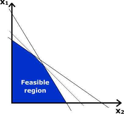 Feasible region for a 2-variable LP problem (Image: en:User:Jacj, Public domain, via Wikimedia Commons)
Based on the PU BBA (PU) syllabus for Business Mathematics II, unit 9.
Discussion
Loading…