Business StatisticsUnit 108 min read

Index Numbers and Time Series – Key Concepts

Unit 10 of Business Statistics: covers index numbers (price, quantity, chain, Laspeyres, Paasche, Fisher) and time series analysis (components, decomposition, forecasting methods) with practical examples and real‑world applications.

Padhai · Based on the official syllabus and past papers
Updated 6 Oct 2026

Key points

Index numbers transform raw data into comparable units, enabling measurement of inflation, growth, and price changes.
Laspeyres, Paasche, and Fisher indices differ in base‑weight choice, affecting sensitivity to price and quantity changes.
Time series data are decomposed into trend, seasonal, cyclical, and irregular components for clearer interpretation.
Forecasting techniques (naïve, moving average, exponential smoothing, ARIMA) provide progressively sophisticated predictions.
Understanding index construction and time‑series decomposition is essential for business planning, policy analysis, and investment decisions.

1. Introduction to Index Numbers

Index numbers are dimensionless ratios that express the relative change of a variable over time or across entities. They are expressed as a percentage of a base value (100).

1.1 Types of Index Numbers

Index Type	Formula	Typical Use	Example
Price Index	$I_{P} = \frac{\sum p _{t} q _{0}}{\sum p _{0} q _{0}} \times 100$	Inflation measurement	Consumer Price Index (CPI)
Quantity Index	$I_{Q} = \frac{\sum p _{0} q _{t}}{\sum p _{0} q _{0}} \times 100$	Output growth	Industrial production index
Chain Index	$I_{c hain} = \prod_{t = 1}^{T} \frac{\sum p _{t} q _{t - 1}}{\sum p _{t - 1} q _{t - 1}} \times 100$	Continuous growth	GDP growth rate
Laspeyres Index	$I_{L} = \frac{\sum p _{t} q _{0}}{\sum p _{0} q _{0}} \times 100$	Fixed‑basket price index	CPI (Laspeyres)
Paasche Index	$I_{P} = \frac{\sum p _{t} q _{t}}{\sum p _{0} q _{t}} \times 100$	Current‑basket price index	CPI (Paasche)
Fisher Index	$I_{F} = I_{L} \times I_{P}$	Combines Laspeyres & Paasche	CPI (Fisher)

Note: $p_{t}, p_{0}$ are prices at time $t$ and base time 0; $q_{t}, q_{0}$ are quantities.

1.2 Worked Example – CPI Calculation

Suppose a basket of 3 goods (rice, milk, bread) has the following prices and quantities in 2020 (base year) and 2021:

Good	2020 Price ( $p_{0}$ )	2020 Quantity ( $q_{0}$ )	2021 Price ( $p_{1}$ )	2021 Quantity ( $q_{1}$ )
Rice	30	100	33	110
Milk	50	50	55	55
Bread	40	80	42	70

Laspeyres CPI (2021)
$I_{L} = \frac{( 33 \times 100 ) + ( 55 \times 50 ) + ( 42 \times 80 )}{( 30 \times 100 ) + ( 50 \times 50 ) + ( 40 \times 80 )} \times 100$ $I_{L} = \frac{3300 + 2750 + 3360}{3000 + 2500 + 3200} \times 100 = \frac{9410}{8700} \times 100 \approx 108.1$

Paasche CPI (2021)
$I_{P} = \frac{( 33 \times 110 ) + ( 55 \times 55 ) + ( 42 \times 70 )}{( 30 \times 110 ) + ( 50 \times 55 ) + ( 40 \times 70 )} \times 100$ $I_{P} = \frac{3630 + 3025 + 2940}{3300 + 2750 + 2800} \times 100 = \frac{9595}{8850} \times 100 \approx 108.5$

Fisher CPI (2021)
$I_{F} = 108.1 \times 108.5 \approx 11725.85 \approx 108.3$

Interpretation: Prices increased by about 8.3 % from 2020 to 2021.

1.3 Chain Index – Continuous Growth

Chain indices link successive periods, allowing for changing baskets. For GDP, the chain index is computed as the product of growth rates between consecutive years.

2. Time Series Analysis

A time series is a sequence of observations recorded at regular intervals (daily, monthly, quarterly). Understanding its structure is essential for forecasting and policy analysis.

2.1 Components of a Time Series

Component	Description	Typical Pattern
Trend	Long‑term direction (upward/downward)	Slow, monotonic change
Seasonality	Regular periodic fluctuations	Peaks in specific months
Cyclical	Long‑term oscillations (2–10 yr)	Business cycles
Irregular	Random noise	Unpredictable shocks

Additive Model: $Y_{t} = T_{t} + S_{t} + C_{t} + I_{t}$
Multiplicative Model: $Y_{t} = T_{t} \times S_{t} \times C_{t} \times I_{t}$

2.2 Decomposition – A Step‑by‑Step Process

flowchart TD
  "Collect Data" --> "Detrend"
  "Detrend" --> "Seasonal Adjustment"
  "Seasonal Adjustment" --> "Extract Cyclical"
  "Extract Cyclical" --> "Identify Irregular"

Detrending: Remove trend using moving averages or regression.
Seasonal Adjustment: Divide or subtract seasonal component.
Cyclical Extraction: Apply low‑pass filters or smoothing.
Irregular: Residual after removing other components.

2.3 Forecasting Methods

Method	Formula	Strengths	Weaknesses
Naïve	$\hat{Y}_{t + 1} = Y_{t}$	Simple, no parameters	Ignores trend/seasonality
Moving Average	$\hat{Y}_{t + 1} = \frac{1}{k} \sum_{i = 0}^{k - 1} Y_{t - i}$	Smooths noise	Requires choice of $k$
Exponential Smoothing	$\hat{Y}_{t + 1} = α Y_{t} + (1 - α) \hat{Y}_{t}$	Captures trend, adjustable smoothing	Sensitive to $α$
Holt’s Linear Trend	$\hat{Y}_{t + 1} = ℓ_{t} + b_{t}$ with $ℓ_{t} = α Y_{t} + (1 - α) (ℓ_{t - 1} + b_{t - 1})$	Handles trend	No seasonality
Holt‑Winters (Seasonal)	Adds seasonal component	Handles trend & seasonality	Requires more parameters
ARIMA	$ϕ (B) (1 - B)^{d} Y_{t} = θ (B) ε_{t}$	Flexible, statistical inference	Complex, requires stationarity

Worked Example – Forecasting Next Month Sales

Monthly sales (in lakhs) for 12 months:

Month	Sales
Jan	120
Feb	130
Mar	125
Apr	140
May	150
Jun	160
Jul	155
Aug	165
Sep	170
Oct	180
Nov	190
Dec	200

Step 1: Compute 3‑month moving average (MA3)
For Jan–Mar: $(120 + 130 + 125) /3 = 125$
For Feb–Apr: $(130 + 125 + 140) /3 = 131.67$
…and so on.

Step 2: Forecast for next month (Jan of next year)
Using MA3 of Oct–Dec: $(180 + 190 + 200) /3 = 190$ .
So forecasted sales for Jan next year = 190 lakhs.

3. Comparison of Index Number Methods

Feature	Laspeyres	Paasche	Fisher
Basket	Base‑year quantities	Current‑year quantities	Combines both
Price Sensitivity	Overestimates inflation if new goods enter	Underestimates inflation if prices rise	Balanced
Data Requirement	Base‑year prices & quantities	Current‑year prices & quantities	Both
Use in Policy	CPI (Laspeyres)	CPI (Paasche)	CPI (Fisher)
Typical Bias	Positive bias (substitution effect ignored)	Negative bias	Minimal bias

4. In the Real World

eSewa – Transaction Fees Index
Idea Used: Price index (Laspeyres) to monitor fee changes across transaction types.
How: Base basket of transaction categories (e.g., bill payment, mobile recharge) with 2020 fees; 2021 fees updated to compute fee inflation.
Daraz – Sales Growth Index
Idea Used: Quantity index to measure growth in total sales volume.
How: Base year sales volume of all product categories; current year volume compared to compute growth rate.
NEPSE – Stock Market Index (NEPSE Index)
Idea Used: Chain index to reflect continuous price changes of listed stocks.
How: Weighted average of stock prices, updated daily; chain index captures compounded growth.
Kathmandu Traffic Routes – Seasonal Traffic Index
Idea Used: Time‑series decomposition to forecast peak traffic periods.
How: Monthly vehicle counts decomposed into trend and seasonality; forecasted using Holt‑Winters to plan road maintenance.

5. Advantages and Disadvantages

Concept	Advantages	Disadvantages
Index Numbers	Simple comparison, policy relevance, standardization	Sensitive to basket choice, substitution bias
Chain Index	Reflects changing baskets, continuous growth	Requires frequent updates, complex computation
Time Series Decomposition	Clarifies underlying patterns, aids forecasting	Requires sufficient data, may misclassify components
Exponential Smoothing	Adaptive, handles trend	Parameter selection critical, may lag
ARIMA	Statistically rigorous, handles autocorrelation	Requires stationarity, complex to estimate

6. Exam Tip

Understand the formulas: Be able to write and explain Laspeyres, Paasche, Fisher, and chain indices.
Practice calculations: Work through at least one CPI example and one time‑series forecast.
Know the components: Be able to label trend, seasonal, cyclical, irregular parts of a series.
Compare methods: Memorize key differences between forecasting techniques (naïve, MA, exponential, ARIMA).
Real‑world application: Relate each concept to a Nepali company or everyday scenario; this often appears in short answer questions.

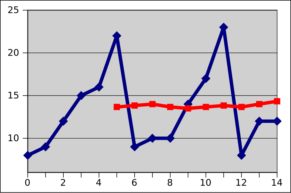moving average chart 3‑month moving average forecast for retail sales (Image: Joxemai, CC BY-SA 3.0, via Wikimedia Commons)

Based on the PU BBA (PU) syllabus for Business Statistics, unit 10.

Discussion

Loading…

Month	Sales
Jan	120
Feb	130
Mar	125
Apr	140
May	150
Jun	160
Jul	155
Aug	165
Sep	170
Oct	180
Nov	190
Dec	200

Month	Sales
Jan	120
Feb	130
Mar	125
Apr	140
May	150
Jun	160
Jul	155
Aug	165
Sep	170
Oct	180
Nov	190
Dec	200

Month	Sales
Jan	120
Feb	130
Mar	125
Apr	140
May	150
Jun	160
Jul	155
Aug	165
Sep	170
Oct	180
Nov	190
Dec	200