Data Analysis and ModelingUnit 68 min read
Regression Modelling: Types, Assumptions, and Applications
Unit 6 of Data Analysis and Modeling explores regression modeling—how to predict relationships between variables, test assumptions, and apply linear/logistic regression in business. Learn formulas, diagnostics, and real-world uses in finance, marketing, and operations.
TAKEAWAYS:
- Regression models predict outcomes by fitting a line (linear) or curve (nonlinear) to data, with R² measuring fit quality.
- Linear regression assumes linearity, independence, homoscedasticity, and normality; violations require transformations or robust methods.
- Logistic regression models binary outcomes (e.g., "buy/no-buy") using probabilities via the logit link function.
- Multicollinearity (correlated predictors) inflates coefficient variance; use VIF or stepwise selection to mitigate it.
- Residual analysis (plots of residuals vs. fitted values) detects heteroscedasticity, outliers, or nonlinearity.
- Businesses use regression for pricing (Daraz), risk (banks), and demand forecasting (NTC).
What is Regression Modeling?
Regression modeling predicts a dependent variable (Y) using one or more independent variables (X₁, X₂, ...). It answers:
- "How does advertising spend (X) affect sales (Y)?"
- "What factors influence loan defaults?"
Key Types
Linear Regression
- Models a linear relationship:
- Simple linear: 1 predictor (e.g., house price vs. size).
- Multiple linear: ≥2 predictors (e.g., salary vs. experience + education).
Logistic Regression
- Models binary outcomes (e.g., "churn/no-churn") using probabilities:
- Outputs odds ratios (e.g., "A 1% increase in ad spend doubles churn odds").
Nonlinear Regression
- Fits curves (e.g., polynomial, exponential) when relationships are nonlinear.
- Example: Gompertz growth model for population trends.
How Linear Regression Works: Step-by-Step
1. Model Assumptions
Regression relies on 4 critical assumptions (violations require fixes):
| Assumption | What It Means | How to Check | Fix if Violated |
|---|---|---|---|
| Linearity | Relationship between X and Y is linear. | Scatter plot, residual plot. | Transform X/Y (log, square root). |
| Independence | Observations are not correlated. | Durbin-Watson test (1.5–2.5 is ideal). | Use time-series models (ARIMA). |
| Homoscedasticity | Residuals have constant variance. | Residual vs. fitted plot (funnel shape = bad). | Weighted least squares (WLS). |
| Normality | Residuals are normally distributed. | Q-Q plot, histogram. | Robust standard errors or bootstrapping. |
2. Estimating Coefficients
Use Ordinary Least Squares (OLS) to minimize the sum of squared residuals (SSR): Example: Predicting monthly sales (Y) of a Daraz seller based on ad spend (X₁) and seasonality (X₂).
| Month | Sales (Y) | Ad Spend (X₁) | Seasonality (X₂) |
|---|---|---|---|
| Jan | 500 | 2000 | 0.8 |
| Feb | 600 | 2500 | 0.9 |
| ... | ... | ... | ... |
Model:
- Interpretation:
- A ₹1,000 increase in ad spend raises sales by ₹200.
- A 0.1 increase in seasonality (e.g., festival month) raises sales by ₹15.
Visualizing Regression
1. Residual Plots (Diagnostics)
graph LR
    A["Scatter Plot: Y vs. X"] --> B["Residual Plot: Residuals vs. Fitted"]
    B --> C["Normal Q-Q Plot"]
B --> D["Homoscedasticity Check"]- Good fit: Residuals randomly scatter around 0.
- Bad fit: Patterns (curves, funnels) → nonlinearity or heteroscedasticity.
2. Real-World Example: NTC’s Revenue Prediction
Problem: NTC wants to predict monthly revenue (Y) using:
- Number of subscribers (X₁)
- Average call duration (X₂)
Data:
| Month | Revenue (Y) | Subscribers (X₁) | Avg. Duration (X₂) |
|---|---|---|---|
| Jan | 800M | 5M | 120 sec |
| Feb | 950M | 5.2M | 130 sec |
Model:
- Prediction for March: 5.5M subscribers, 140 sec duration → .
Logistic Regression: Binary Outcomes
How It Works
- Outputs probabilities (0 to 1) using the logit link:
- Example: Predicting if a Khalti user will default on a loan based on:
- Income (X₁)
- Loan amount (X₂)
Model:
- Interpretation:
- A ₹10,000 increase in income reduces default odds by 5% (since ).
- A ₹100,000 loan increases default odds by 30% (since ).
Common Pitfalls and Fixes
| Issue | Cause | Solution |
|---|---|---|
| Multicollinearity | Predictors are highly correlated. | Remove one, use PCA, or VIF < 5. |
| Overfitting | Too many predictors. | Use stepwise regression or cross-validation. |
| Outliers | Extreme values skew results. | Winsorize data or use robust regression. |
| Nonlinearity | Relationship is curved. | Add polynomial terms (e.g., ). |
## In the Real World
Daraz’s Demand Forecasting
- Uses multiple linear regression to predict product demand based on:
- Price (X₁)
- Seasonality (X₂)
- Competitor promotions (X₃)
- Example: If Daraz lowers the price of a laptop by ₹5,000, sales increase by 12% (coefficient ).
- Uses multiple linear regression to predict product demand based on:
Ncell’s Churn Prediction
- Uses logistic regression to identify customers likely to cancel:
- Call duration (X₁)
- Data usage (X₂)
- Customer service complaints (X₃)
- Example: A user with <100 mins/month** and **>3 complaints has a 70% chance of churning.
- Uses logistic regression to identify customers likely to cancel:
Nepal Rastra Bank’s Loan Risk
- Banks use probit/logit models to assess loan defaults:
- Borrower income (X₁)
- Loan-to-value ratio (X₂)
- Credit history (X₃)
- Example: A borrower with a 60% LTV and poor credit has a 40% default probability.
- Banks use probit/logit models to assess loan defaults:
## Exam Tip
Always check assumptions before interpreting results. Examiners test this!
- Plot residuals vs. fitted values.
- Use Durbin-Watson for autocorrelation.
Interpret coefficients correctly:
- Linear: "A 1-unit increase in X → Y changes by ."
- Logistic: "A 1-unit increase in X → odds of Y change by ."
Compare models using:
- R² (higher = better fit, but can overfit).
- Adjusted R² (penalizes extra predictors).
- AIC/BIC (for nonlinear models).
Real-world applications are gold:
- Link regression to business decisions (e.g., "NTC should increase rates by 5% to boost revenue by ₹200M").
- Use Nepali examples (Ncell, Daraz, banks) to stand out.
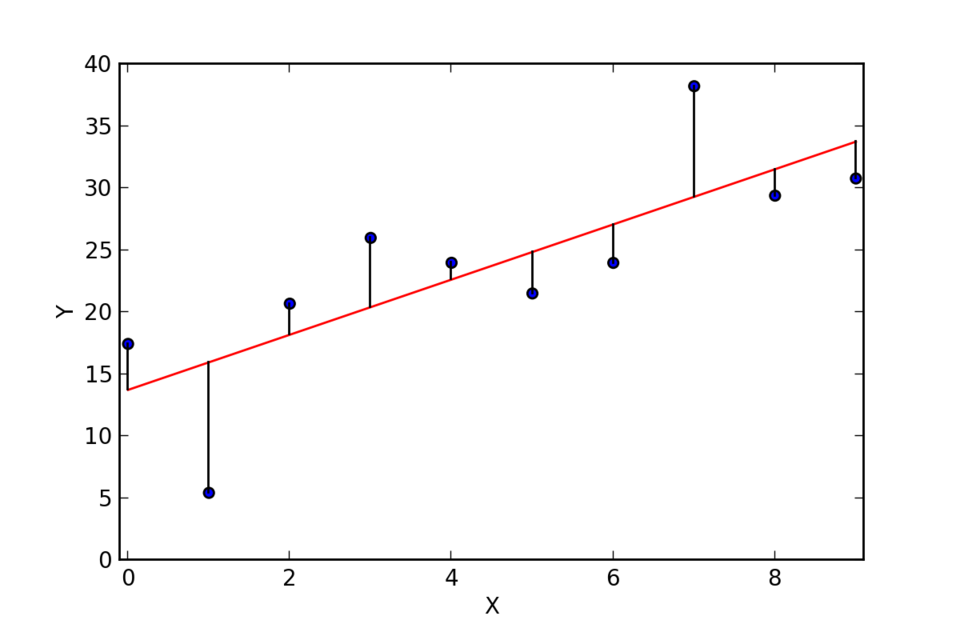 Example: House price vs. size in Kathmandu (Image: Thomas.haslwanter, CC BY-SA 3.0, via Wikimedia Commons)
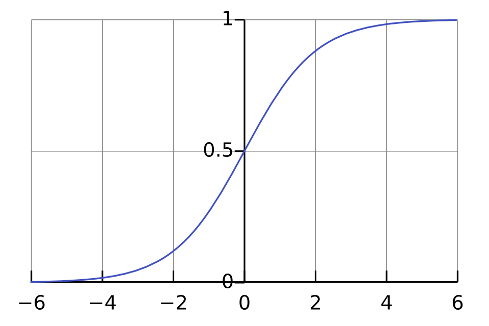 Example: Khalti loan default probability (Image: Qef (talk), Public domain, via Wikimedia Commons)
graph TD
A["Collect Data"] --> B["Check Assumptions"]
B --> C["Fit Model (OLS/Logit)"]
C --> D["Diagnose Residuals"]
D -->|"Good"| E["Interpret Coefficients"]
D -->|"Bad"| F["Transform Data or Use Robust Methods"]
E --> G["Make Predictions"]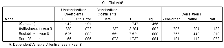 Example: Daraz sales model output (Image: Jtneill, Public domain, via Wikimedia Commons)
Based on the PU BBA (PU) syllabus for Data Analysis and Modeling, unit 6.
Discussion
Loading…