Higher Order Linear Differential Equations: Methods, Solutions & Applications

TAKEAWAYS:

• Higher-order linear ODEs are solved by finding characteristic equations (for constant-coefficient cases) or using power series (for variable coefficients like Bessel’s equation).
• Homogeneous equations have solutions built from roots of the characteristic equation; nonhomogeneous solutions require a particular solution (guess-and-check or variation of parameters).
• Reduction of order converts a 2nd-order ODE into a 1st-order ODE if one solution is known.
• Bessel’s equation and Legendre’s equation are special cases with series solutions tied to physics (vibrations, heat) and engineering (wave propagation).
• Exam focus: Memorize standard forms, characteristic equation roots (real/distinct, real/repeated, complex), and when to use each method.

---

1. Classification and General Form

Higher-order linear ODEs extend 1st-order equations to describe systems with acceleration, jerk, or higher derivatives. The general form is: $$a_n(x)\frac{d^{n}y}{d{x}^n}+a_{n-1}(x)\frac{d^{n-1}y}{d{x}^{n-1}}+\cdots +a_1(x)\frac{dy}{dx}+a_0(x)y=g(x).$$

• Order: Highest derivative (e.g., $y^{\prime \prime }$ is 2nd order).
• Linearity: Superposition applies; solutions can be added/scaled.
• Homogeneous: $g(x)=0$. Solutions are complementary ($y_c$).
• Nonhomogeneous: $g(x)\ne 0$. Solution = $y_c+y_p$ (particular solution).

Visual: Classification Tree

---

2. Constant-Coefficient Homogeneous Equations

For equations like: $$y^{\prime \prime }+a{y}^{\prime }+by=0,$$ assume $y=e^{rx}$ and solve the characteristic equation: $$r^2+ar+b=0.$$ Roots determine the general solution:

Worked Example 1: Real Repeated Roots

Solve $y^{\prime \prime }-6y^{\prime }+9y=0$.

1. Characteristic equation: $r^2-6r+9=0$ → $(r-3{)}^2=0$ → $r=3$ (repeated).
2. General solution: $y_c=(c_1+c_{2}x)e^{3x}$.

Real-World Link: Damped Oscillations in a Spring

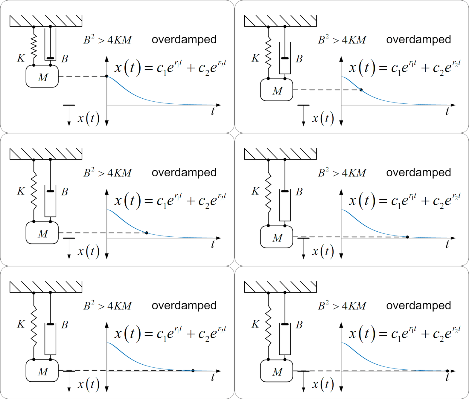A mechanical system with a mass $m$, spring $k$, and damper $c$ obeys $m{y}^{\prime \prime }+c{y}^{\prime }+ky=0$. For critical damping ($c=2\sqrt{mk}$), the roots are real and repeated, leading to a solution like $y(t)=(c_1+c_{2}t)e^{-\gamma t}$, where $\gamma =c/(2m)$. This describes how a car’s suspension or NTC’s power grid stabilizers return to equilibrium without oscillation. (Image: Guillermo Bossio, CC BY-SA 4.0, via Wikimedia Commons)

---

3. Nonhomogeneous Equations: Methods

A. Undetermined Coefficients

For $g(x)$ like polynomials, exponentials, sines/cosines, guess a form for $y_p$:

Worked Example 2: Polynomial Nonhomogeneous Term Solve $y^{\prime \prime }-y^{\prime }-2y=3x+1$.

1. Complementary solution: $y_c=c_1{e}^{2x}+c_2{e}^{-x}$.
2. Guess for $y_p$: $y_p=Ax+B$ (since $g(x)=3x+1$).
3. Derivatives: $y_p^{\prime }=A$, $y_p^{\prime \prime }=0$. Substitute into ODE: $$0-A-2(Ax+B)=3x+1⟹-2Ax-A-2B=3x+1.$$
4. Equate coefficients: $$-2A=3⟹A=-\frac{3}{2},-A-2B=1⟹B=\frac{1}{4}.$$
5. General solution: $$y=c_1{e}^{2x}+c_2{e}^{-x}-\frac{3}{2}x+\frac{1}{4}.$$

B. Variation of Parameters

For nonhomogeneous terms not covered by undetermined coefficients (e.g., $g(x)=\ln x$), use: $$y_p=-y_1(x)\int \frac{y_2(x)g(x)}{W(y_1,y_2)}dx+y_2(x)\int \frac{y_1(x)g(x)}{W(y_1,y_2)}dx,$$ where $W$ is the Wronskian: $$W(y_1,y_2)=y_1{y}_2^{\prime }-y_2{y}_1^{\prime }.$$

Worked Example 3: Variation of Parameters Solve $y^{\prime \prime }+y=\tan x$ with $y_c=c_1\cos x+c_2\sin x$.

1. Wronskian: $W={\cos }^{2}x+{\sin }^{2}x=1$.
2. Particular solution: $$y_p=-\cos x\int \sin x\cdot \tan xdx+\sin x\int \cos x\cdot \tan xdx.$$
3. Simplify integrals: $$\int \sin x\tan xdx=\int {\sin }^{2}x/\cos xdx=\int (1-{\cos }^{2}x)/\cos xdx=\tan x-\sec x+C,$$ $$\int \cos x\tan xdx=\int \sin xdx=-\cos x+C.$$
4. Thus: $$y_p=-\cos x(\tan x-\sec x)+\sin x(-\cos x)=-\cos x\tan x+\cos x\sec x-\sin x\cos x.$$ Simplify using $\tan x=\sin x/\cos x$ and $\sec x=1/\cos x$: $$y_p=-\sin x+1-\sin x\cos x.$$

Real-World Link: Electric Circuit Analysis (NTC Grid)

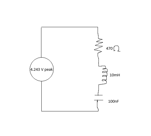In an RLC circuit, the voltage $V(t)$ across a resistor-inductor-capacitor network satisfies: (Image: Nkkoy, CC0, via Wikimedia Commons) $$L\frac{d^{2}Q}{d{t}^2}+R\frac{dQ}{dt}+\frac{1}{C}Q=V_0\sin \omega t.$$ Here, $Q$ is charge, and the nonhomogeneous term $V_0\sin \omega t$ represents an AC source (like Nepal’s 220V supply). The particular solution $y_p$ describes the steady-state response, critical for designing NTC’s power distribution systems to avoid resonance (which can cause blackouts).

---

4. Reduction of Order

If one solution $y_1$ is known, reduce the 2nd-order ODE to a 1st-order ODE for $y_2$: $$y=v(x)y_1(x),y^{\prime }=v^{\prime }{y}_1+v{y}_1^{\prime },y^{\prime \prime }=v^{\prime \prime }{y}_1+2v^{\prime }{y}_1^{\prime }+v{y}_1^{\prime \prime }.$$ Substitute into the ODE to solve for $v(x)$.

Worked Example 4: Reduction of Order Given $y^{\prime \prime }-4y^{\prime }+4y=0$ with $y_1=e^{2x}$, find a second solution.

1. Assume $y=v{e}^{2x}$.
2. Compute derivatives: $$y^{\prime }=v^{\prime }{e}^{2x}+2v{e}^{2x},y^{\prime \prime }=v^{\prime \prime }{e}^{2x}+4v^{\prime }{e}^{2x}+4v{e}^{2x}.$$
3. Substitute into ODE: $$(v^{\prime \prime }+4v^{\prime }+4v)e^{2x}-4(v^{\prime }+2v)e^{2x}+4v{e}^{2x}=0⟹v^{\prime \prime }{e}^{2x}=0.$$
4. Thus, $v^{\prime \prime }=0⟹v=c_{1}x+c_2$.
5. Second solution: $y_2=x{e}^{2x}$ (take $c_1=1,c_2=0$).

Real-World Link: Traffic Flow Modeling (Kathmandu Roads)

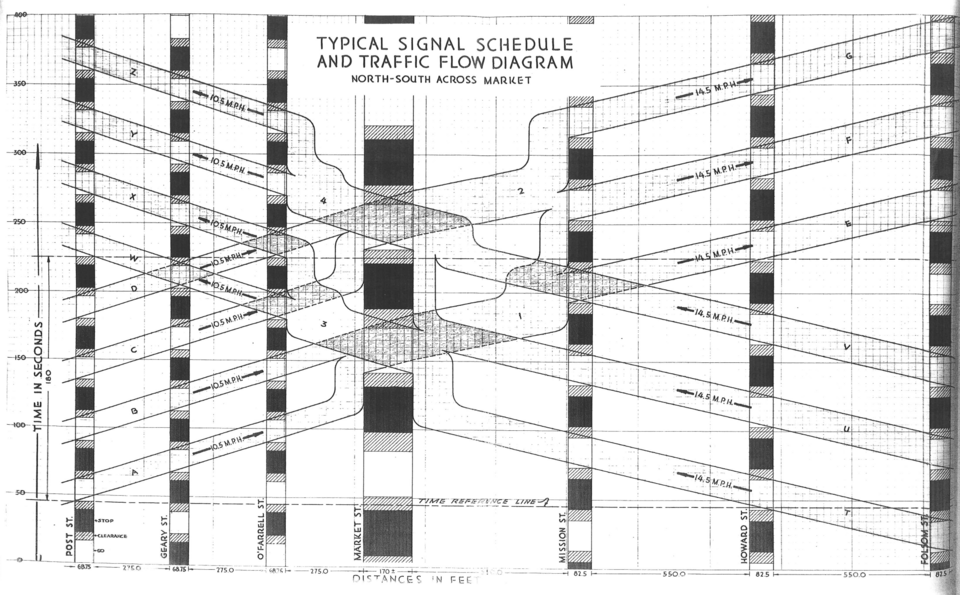In traffic engineering, the Lighthill-Whitham-Richards (LWR) model uses 2nd-order PDEs to describe car density $\rho (x,t)$. If one solution (e.g., ${\rho }_1(x,t)=\text{constant}$) is known, reduction of order helps find another solution representing shock waves or jam propagation. For example, during Dashain, the sudden increase in traffic on Ring Road can be modeled by adding a particular solution to the homogeneous flow. (Image: City of San Francisco, CC BY-SA 3.0, via Wikimedia Commons)

---

5. Special Functions: Bessel’s and Legendre’s Equations

A. Bessel’s Equation

$$x^2{y}^{\prime \prime }+x{y}^{\prime }+(x^2-n^2)y=0.$$ Solutions: Bessel functions $J_n(x)$ and $Y_n(x)$ (for integer $n$): $$y=c_1{J}_n(x)+c_2{Y}_n(x).$$ Graphs:

B. Legendre’s Equation

$$(1-x^2)y^{\prime \prime }-2x{y}^{\prime }+n(n+1)y=0.$$ Solutions: Legendre polynomials $P_n(x)$ (Rodrigues form): $$P_n(x)=\frac{1}{2^{n}n!}\frac{d^n}{d{x}^n}(x^2-1{)}^n.$$ Worked Example 5: Legendre Polynomial Find $P_2(x)$: $$P_2(x)=\frac{1}{8}\frac{d^2}{d{x}^2}(x^2-1{)}^2=\frac{1}{8}\frac{d}{dx}[4x(x^2-1)]=\frac{1}{8}[4(x^2-1)+8x^2]=\frac{3x^2-1}{2}.$$

Real-World Link: Quantum Mechanics and NEPSE Stock Prices

1. Bessel Functions: Used in vibration analysis of NTC transmission towers (modeling stress as a function of radius $x$).
2. Legendre Polynomials: In quantum mechanics, they describe electron orbitals in atoms. In finance, they approximate stock price correlations (e.g., NEPSE’s sector-wise movements can be modeled using Legendre expansions for risk analysis).

---

6. Series Solutions (Frobenius Method)

For equations with variable coefficients (e.g., $y^{\prime \prime }+p(x)y^{\prime }+q(x)y=0$), assume a power series: $$y=\sum _{k=0}^{\infty }{a}_k{x}^{k+r}.$$ Steps:

1. Substitute into the ODE.
2. Collect like terms to find indicial equation (for $a_0$).
3. Solve for recurrence relations.

Worked Example 6: Series Solution Solve $2x^2{y}^{\prime \prime }+x{y}^{\prime }+(x^2-1)y=0$.

1. Assume $y=\sum a_k{x}^{k+r}$.
2. Compute derivatives: $$y^{\prime }=\sum (k+r)a_k{x}^{k+r-1},y^{\prime \prime }=\sum (k+r)(k+r-1)a_k{x}^{k+r-2}.$$
3. Substitute into ODE: $$2\sum (k+r)(k+r-1)a_k{x}^{k+r}+\sum (k+r)a_k{x}^{k+r}+\sum a_k{x}^{k+r+2}-\sum a_k{x}^{k+r}=0.$$
4. Indicial equation (coefficient of $x^r$): $$2r(r-1)+r-1=0⟹r^2-1=0⟹r=\pm 1.$$
5. For $r=1$: $$a_1=0,a_2=\frac{a_0}{6},a_3=0,a_4=\frac{a_0}{180},\dots$$ Thus: $$y_1=x\left(1+\frac{x^2}{6}+\frac{x^4}{180}+\dots \right).$$
6. For $r=-1$ (logarithmic term appears): $$y_2=y_1\ln x+\sum b_k{x}^{k-1}.$$

Real-World Link: Heat Equation in Semiconductors

---

Exam Tip

1. Memorize standard forms: Know when to use characteristic equations, undetermined coefficients, variation of parameters, and reduction of order.
2. Check for overlaps: If your guess for $y_p$ matches a term in $y_c$, multiply by $x$ (e.g., guess $Ax{e}^{ax}$ instead of $A{e}^{ax}$).
3. Practice Bessel/Legendre: For series solutions, focus on the indicial equation and recurrence relations. In exams, you may be asked to compute the first few terms.
4. Real-world connections: Questions may link ODEs to circuits (NTC), mechanical systems (Ncell towers), or finance (NEPSE). Relate your answers to these contexts.
5. Graphs are key: Always sketch the characteristic roots’ behavior (e.g., damped oscillations for complex roots) and Bessel/Legendre function graphs to visualize solutions.

---

Summary Table: Solution Methods