Vector Calculus – Fields, Integrals, and Theorems

Definitions

Vector field $\mathbf{F}:{\mathbb{R}}^3\to {\mathbb{R}}^3$ assigns a vector $\mathbf{F}(x,y,z)=(P,Q,R)$ to each point $(x,y,z)$.
Scalar field $f:{\mathbb{R}}^3\to \mathbb{R}$ assigns a single real number to each point.

Gradient
$$\nabla f=\left(\frac{\partial f}{\partial x},\frac{\partial f}{\partial y},\frac{\partial f}{\partial z}\right)$$
Points in the direction of greatest increase of $f$.

Divergence
$$\nabla \cdot \mathbf{F}=\frac{\partial P}{\partial x}+\frac{\partial Q}{\partial y}+\frac{\partial R}{\partial z}$$
Measures net flux per unit volume.

Curl
$$\nabla \times \mathbf{F}=\left(\frac{\partial R}{\partial y}-\frac{\partial Q}{\partial z},\frac{\partial P}{\partial z}-\frac{\partial R}{\partial x},\frac{\partial Q}{\partial x}-\frac{\partial P}{\partial y}\right)$$
Measures local rotation.

Line integral of a vector field along a curve $C$ parametrised by $\mathbf{r}(t)$, $a\le t\le b$:
$${\int }_C\mathbf{F}\cdot d\mathbf{r}={\int }_a^b\mathbf{F}(\mathbf{r}(t))\cdot {\mathbf{r}}^{\prime }(t)dt$$

Surface integral of a vector field over an oriented surface $S$ with unit normal $\mathbf{n}$:
$${\iint }_S\mathbf{F}\cdot d\mathbf{S}={\iint }_S\mathbf{F}\cdot \mathbf{n}dS$$

Flux of $\mathbf{F}$ through $S$ is the surface integral of $\mathbf{F}\cdot \mathbf{n}$.

Gradient, Divergence, and Curl

Visualising a Vector Field

The arrows rotate counter‑clockwise, indicating a rotational field with zero divergence.

Gradient Field Example

The gradient vectors point radially outward, perpendicular to the level curves.

Divergence and Curl Illustration

The first field has uniform outward flux; the second field is irrotational.

Line Integrals

Line integrals measure work done by a force field or circulation of a fluid.

Step‑by‑Step Procedure (Mermaid)

flowchart TD
  A["Define vector field F"] --> B["Choose path C"]
  B --> C["Parameterise C: r(t)"]
  C --> D["Compute r'(t)"]
  D --> E["Evaluate F(r(t)) · r'(t)"]
  E --> F["Integrate over t"]
  F --> G["Result: line integral"]

Worked Example – Circulation of a Rotational Field

Problem: Compute
$${\oint }_C\mathbf{F}\cdot d\mathbf{r},\mathbf{F}(x,y)=(y,-x),C:x^2+y^2=1$$
Solution:
Parametrise $C$ by $\mathbf{r}(t)=(\cos t,\sin t)$, $0\le t\le 2\pi$.
$${\mathbf{r}}^{\prime }(t)=(-\sin t,\cos t)$$
$$\mathbf{F}(\mathbf{r}(t))=(\sin t,-\cos t)$$
Dot product:
$$\mathbf{F}\cdot {\mathbf{r}}^{\prime }=(\sin t)(-\sin t)+(-\cos t)(\cos t)=-{\sin }^{2}t-{\cos }^{2}t=-1$$
Integral:
$${\int }_0^{2\pi }(-1)dt=-2\pi$$
Result: $-2\pi$.

Real‑world tie‑in: This is the circulation of a velocity field around a vortex in fluid dynamics. The negative sign indicates clockwise rotation, matching the direction of the field.

Visualising the Path and Field

Surface Integrals

Surface integrals compute flux of a vector field through a surface.

Worked Example – Flux Through a Sphere

Problem: Find the flux of $\mathbf{F}(x,y,z)=(x,y,z)$ through the sphere $x^2+y^2+z^2=1$.

Solution:
Use the Divergence Theorem:
$${\iint }_S\mathbf{F}\cdot d\mathbf{S}={\iiint }_V\nabla \cdot \mathbf{F}dV$$
Compute divergence:
$$\nabla \cdot \mathbf{F}=1+1+1=3$$
Volume of unit sphere:
$$V=\frac{4}{3}\pi (1{)}^3=\frac{4}{3}\pi$$
Flux:
$$3\times \frac{4}{3}\pi =4\pi$$

Real‑world tie‑in: In electromagnetism, this is analogous to computing the electric flux through a spherical surface surrounding a point charge, yielding $4\pi {ϵ}_0$ times the charge.

Visualising the Surface Integral

Fundamental Theorems

Example Using Stokes’ Theorem

Compute the line integral of $\mathbf{F}=(yz,xz,xy)$ around the boundary of the unit disk in the $xy$-plane.
By Stokes’ Theorem,
$${\oint }_C\mathbf{F}\cdot d\mathbf{r}={\iint }_D(\nabla \times \mathbf{F})\cdot \mathbf{k}dA$$
Curl of $\mathbf{F}$ is $(0,0,0)$, so the integral is $0$.

Advantages and Applications

In the real world

1. Pathao Delivery Routing – The company models traffic flow as a vector field over Kathmandu’s map. The gradient of travel time guides the algorithm to find the steepest descent path, minimizing delivery time.
2. Ncell Signal Strength Mapping – Signal strength is represented as a scalar field. The gradient points toward stronger reception areas, helping users find optimal positions.
3. Google Maps Navigation – Uses vector calculus to compute the shortest path by treating the road network as a surface and applying the divergence theorem to estimate traffic density and adjust routes in real time.

Concrete Example:
A delivery drone in Pathao must fly from point $A$ to $B$ while avoiding no‑fly zones. The drone’s control system models the airspace as a vector field where each vector points toward lower congestion. By integrating the field along a candidate path, the system calculates the total “congestion cost” and selects the path with minimal integral, effectively solving a line integral problem in real time.

Exam tip

• Parametrisation is key: Always write the curve or surface in terms of a parameter before computing integrals.
• Check orientation: For line integrals, the direction of traversal matters; for surface integrals, the normal’s direction matters.
• Use theorems to simplify: Convert a difficult line integral to a double integral via Green’s Theorem, or a surface integral to a volume integral via Divergence Theorem.
• Practice with real‑world data: Work through examples that involve physical fields (electric, magnetic, velocity) to build intuition.
• Verify units: Ensure the integrand’s units match the expected physical quantity (e.g., work, flux).

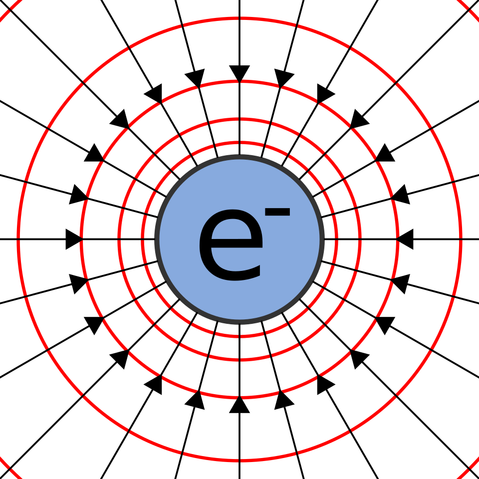Electric field lines around a point charge (Image: Sjlegg, Public domain, via Wikimedia Commons) 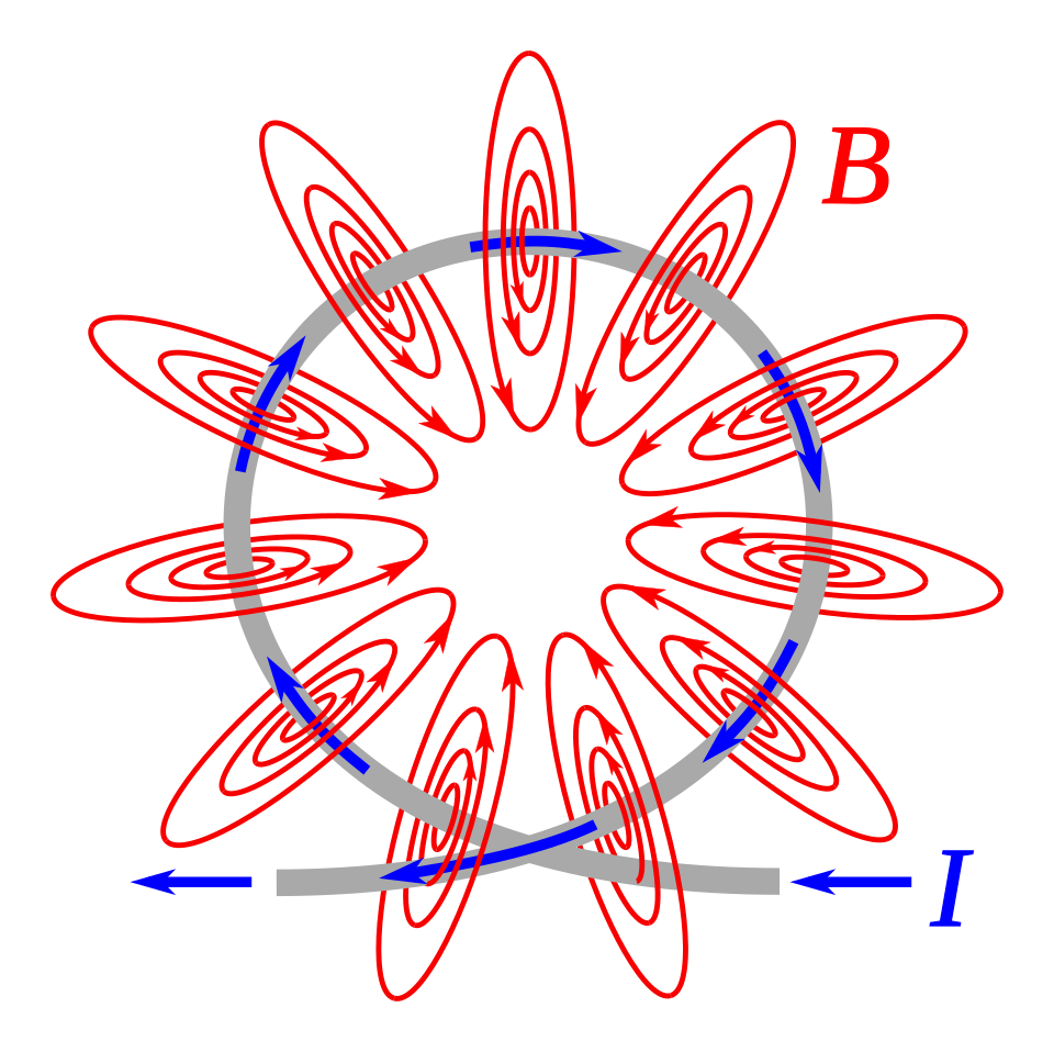Magnetic field lines encircling a wire (Image: Chetvorno, CC0, via Wikimedia Commons)