Machine LearningUnit 912 min read
Neural Networks & Deep Learning: Architectures, Training, and Applications
Unit 9 of Machine Learning explores neural networks (MLPs, CNNs, RNNs), deep learning architectures, backpropagation, activation functions, and real-world applications like image recognition and NLP, with worked examples and exam-focused insights.
TAKEAWAYS:
- Neural networks are computational graphs of interconnected layers (input → hidden → output) that learn patterns via weight adjustments during training.
- Deep learning extends neural networks by stacking multiple hidden layers (e.g., CNNs for images, RNNs for sequences) to model complex hierarchies.
- Backpropagation efficiently computes gradients using the chain rule, enabling layer-wise weight updates via gradient descent.
- Activation functions (ReLU, sigmoid, tanh) introduce non-linearity; loss functions (MSE, cross-entropy) quantify prediction errors.
- Overfitting is mitigated via regularization (dropout, L2), batch normalization, and early stopping.
- Real-world systems (e.g., Google’s AutoML, Pathao’s route optimization) use deep learning for automation, prediction, and decision-making.
Core Concepts: From Perceptrons to Deep Networks
1. Neural Networks: The Building Blocks
A neural network is a directed acyclic graph where:
- Nodes (neurons) compute weighted sums of inputs + bias, then apply an activation function.
- Layers transform data hierarchically:
- Input layer: Raw features (e.g., pixel values for an image).
- Hidden layers: Learn abstract representations (e.g., edges → textures → objects).
- Output layer: Produces predictions (e.g., class probabilities).
graph LR
    A["Input Layer (784 neurons)"] --> B["Hidden Layer 1 (256 neurons, ReLU)"]
    B --> C["Hidden Layer 2 (128 neurons, ReLU)"]
    C --> D["Output Layer (10 neurons, Softmax)"]
Why layers?
- A single-layer perceptron can only model linear relationships. Stacking layers creates non-linear decision boundaries (e.g., XOR problem).
2. Activation Functions: Introducing Non-Linearity
Activation functions introduce non-linearity, enabling networks to learn complex patterns. Compare:
| Function | Formula | Output Range | Use Case | Drawback |
|---|---|---|---|---|
| Sigmoid | (0, 1) | Binary classification (output) | Vanishing gradients | |
| Tanh | (-1, 1) | Hidden layers (centered outputs) | Vanishing gradients | |
| ReLU | [0, ∞) | Hidden layers (default choice) | "Dying ReLU" (neurons stuck at 0) | |
| Leaky ReLU | if , else | (-∞, ∞) | Mitigates dying ReLU | Hyperparameter sensitivity |
Visual: ReLU vs. Sigmoid Worked Example: Why ReLU Dominates
- Problem: Train a 2-layer network to classify the XOR gate.
- Sigmoid: Gradients become tiny for large inputs → slow learning.
- ReLU: Sparsity (many zeros) speeds up training; no saturation.
3. Forward and Backward Propagation
Forward Pass: Data → Prediction
For an input , the output is computed as: where:
- : Weights of layer ,
- : Activations from previous layer,
- : Activation function.
Example: Single Neuron
# Pseudocode for one neuron
weight = [0.5, -0.3]  # W
bias = 0.1             # b
input = [1.0, 0.5]     # x

z = weight[0]*input[0] + weight[1]*input[1] + bias  # z = 0.5*1 + (-0.3)*0.5 + 0.1 = 0.4
a = max(0, z)         # ReLU → a = 0.4
Backward Pass: Error → Weight Updates
- Compute Loss: Compare prediction to true label using a loss function (e.g., Mean Squared Error for regression):
- Chain Rule: Propagate error backward to compute gradients for each weight:
- Update Weights: Adjust weights via gradient descent: where is the learning rate.
Visual: Backpropagation Path
graph TD
    A["Loss (L)"] -->|"∂L/∂ŷ"| B["Output Layer"]
    B -->|"∂ŷ/∂z"| C["Weight W"]
    C -->|"∂z/∂W"| D["Update W"]
Worked Example: Backpropagation for a 2-Layer Network Given:
- Input ,
- True label (binary classification),
- Weights: , (hidden layer),
- , (output layer),
- Activation: ReLU (hidden), Sigmoid (output).
Steps:
- Forward Pass:
- Hidden layer: , .
- Output: , .
- Loss: .
- Backward Pass:
- .
- .
- .
- Update : .
Specialized Architectures
1. Convolutional Neural Networks (CNNs): For Spatial Data
CNNs excel at image processing by exploiting local connectivity and parameter sharing via kernels (filters).
Key Components:
- Convolutional Layer: Applies filters to extract features (edges, textures).
- Pooling Layer: Reduces spatial dimensions (e.g., max-pooling).
- Fully Connected Layer: Classifies features.
Example: Edge Detection Real-World Use: Google Photos uses CNNs to auto-tag images (e.g., "Mount Everest") by detecting objects/landmarks.
2. Recurrent Neural Networks (RNNs): For Sequential Data
RNNs process sequences (time series, text) by maintaining a hidden state : Problem: Vanishing gradients for long sequences → LSTMs/GRUs solve this.
Example: Sentiment Analysis
graph LR
    A["Input: 'I love ML!'"] --> B["Word Embeddings"]
    B --> C["RNN Cell (LSTM)"]
    C --> D["Hidden State h_t"]
    D --> E["Output: Positive"]
Real-World Use: Pathao’s chatbot uses RNNs to understand user queries like "Take me to Thapathali" by processing sequential words.
3. Transformers: Attention Is All You Need
Transformers replace RNNs with self-attention, enabling parallel processing: Use Case: Google’s BERT (Bidirectional Encoder Representations) for NLP tasks like translation.
Training Deep Networks
1. Optimization Techniques
| Technique | Idea | When to Use |
|---|---|---|
| Stochastic Gradient Descent (SGD) | Updates weights per training example. | Small datasets. |
| Mini-Batch GD | Updates per batch (e.g., 32 examples). | Balances speed/accuracy. |
| Adam | Combines momentum + adaptive learning rates. | Default choice for most problems. |
| Learning Rate Scheduling | Dynamically adjusts (e.g., reduce on plateau). | Avoid local minima. |
Visual: Loss vs. Epochs
2. Overfitting and Regularization
Symptoms: Model performs well on training data but poorly on test data. Solutions:
| Method | How It Works | Example |
|---|---|---|
| Dropout | Randomly deactivates neurons during training. | Keep probability = 0.5. |
| L2 Regularization | Penalizes large weights: . | . |
| Batch Normalization | Normalizes layer inputs to stabilize training. | , . |
| Early Stopping | Stops training when validation loss plateaus. | Patience = 5 epochs. |
Worked Example: Dropout in a 3-Layer Network
- Without Dropout: All neurons active → co-adaptation → overfitting.
- With Dropout (p=0.5):
- Each training step uses a random subset of neurons.
- Forces network to distribute learning → better generalization.
In the Real World
eSewa’s Fraud Detection
- Idea Used: CNNs + Anomaly Detection
- How: A CNN analyzes transaction patterns (e.g., sudden large payments) to flag fraudulent activities. The network is trained on labeled data (normal vs. fraudulent transactions) and uses autoencoders to detect deviations in new transactions.
- Example: If a user in Kathmandu suddenly transfers ₹50,000 to a new account in India, the CNN’s output layer (with a threshold) triggers an alert.
Pathao’s Route Optimization
- Idea Used: Reinforcement Learning (Deep Q-Networks, DQN)
- How: Pathao’s algorithm treats each ride as a Markov Decision Process (MDP). A neural network (with input: traffic data, rider location, time) outputs the best route. The network is trained via Q-learning, where rewards are based on factors like distance, traffic, and rider satisfaction.
- Example: For a request from Lakshmi Path to Thapathali during peak hours, the DQN might choose a route via Putalisadak to avoid the congested Ring Road, even if it’s slightly longer.
Ncell’s Customer Churn Prediction
- Idea Used: RNNs (LSTM) + Classification
- How: Ncell collects call logs, SMS usage, and payment history to predict which customers might switch to competitors. An LSTM processes sequential data (e.g., "user called customer service 3 times this month"), and the output layer uses a sigmoid activation to predict churn probability (0 to 1).
- Example: If a user’s call duration drops by 40% over 2 weeks and they stop using data roaming, the LSTM’s hidden state evolves to reflect dissatisfaction, and the output predicts a 78% chance of churn.
Exam Tip
What Examiners Look For:
- Architecture Diagrams: Draw and label a 3-layer MLP, CNN with pooling, or LSTM cell. Use arrows for data flow and annotate weights/biases.
- Math Derivations: For backpropagation, show one step of the chain rule (e.g., ) with clear variable definitions.
- Hyperparameter Trade-offs:
- Why use ReLU over sigmoid? → Faster training, no vanishing gradients.
- When to use dropout? → If training loss << validation loss.
- Real-World Mapping:
- Question: "How would you design a system to detect fake news?"
- Answer: Use a Transformer (BERT) for text classification, trained on labeled data (true/false), with attention layers to weigh important words (e.g., "source: XYZ news").
Common Pitfalls:
- Forgetting to normalize input data (e.g., pixel values [0, 255] → [0, 1]).
- Confusing batch size (number of samples per gradient update) with epoch (full passes over the dataset).
- Ignoring vanishing gradients in deep networks → always mention ReLU/LSTM as solutions.
Sample Exam Question: "Explain how a CNN processes a 32×32 grayscale image to classify it as a digit (0–9). Include the role of each layer and the output of the final layer." Expected Answer:
- Input Layer: 32×32 = 1024 neurons (pixel values 0–255).
- Conv Layer 1: 3×3 filters → 28×28 feature maps (edges).
- Pooling: Max-pooling (2×2) → 14×14.
- Conv Layer 2: 5×5 filters → 10×10 feature maps (shapes).
- Flatten: 10×10×64 = 6400 neurons.
- FC Layer: 128 neurons (ReLU) → abstract features.
- Output Layer: 10 neurons (Softmax) → probabilities for digits 0–9.
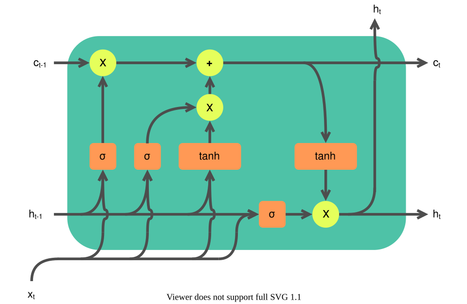 Internal gates (forget, input, output) in an LSTM unit (Image: Original Version: Guillaume Chevalier, Redrawn as SVG by ket, CC BY 4.0, via Wikimedia Commons)
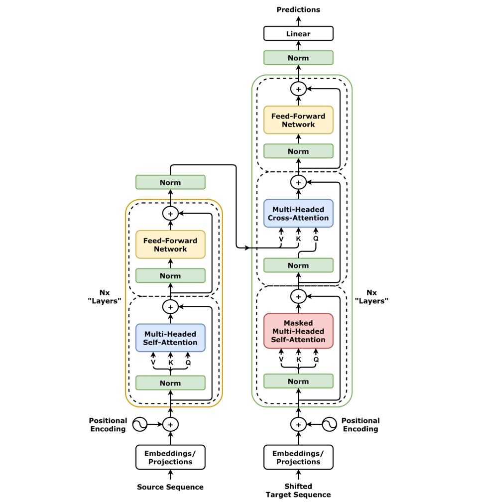 Self-attention mechanism with query/key/value matrices (Image: dvgodoy, CC BY 4.0, via Wikimedia Commons)
Based on the PU BE Computer (PU) syllabus for Machine Learning (CMP364), unit 9.
Discussion
Loading…