Simulation and ModelingUnit 76 min read
Simulation Output Analysis: Confidence Intervals, Hypothesis Testing & Steady-State Detection
Unit 7 of Simulation and Modeling covers how to analyze simulation results statistically—confidence intervals, hypothesis testing, steady-state detection, and output data analysis—with real-world applications in queueing systems, financial models, and system performance evaluation.
Key Concepts & Definitions
1. Simulation Output Data
Simulation output is the data generated from running a simulation model. It can be:
- Terminated output: Data collected over a fixed time period (e.g., simulating a bank’s daily transactions for 8 hours).
- Steady-state output: Data collected after the system reaches equilibrium (e.g., analyzing a hospital’s patient queue after initial fluctuations).
Why analyze output? Raw simulation data is noisy and requires statistical methods to extract meaningful insights.
2. Confidence Intervals for Simulation Output
Confidence intervals (CIs) estimate the range within which the true mean of a simulated metric lies, with a certain probability (e.g., 95%).
How to Compute Confidence Intervals
For a sample mean with standard deviation and sample size :
- : t-distribution critical value (from tables).
- : Sample standard deviation.
- : Number of replications (runs).
Example: Estimating Average Wait Time in a Queue Suppose we simulate a Pathao driver’s pickup queue 30 times, recording average wait times (in minutes):
| Run | Avg Wait Time (min) |
|---|---|
| 1 | 4.2 |
| 2 | 5.1 |
| ... | ... |
| 30 | 3.9 |
Steps:
- Compute min, min.
- For 95% CI, (from t-table).
- Margin of error (ME) = .
- CI = 4.5 ± 0.29 → [4.21, 4.79] min.
Interpretation: We are 95% confident the true average wait time lies between 4.21 and 4.79 minutes.
3. Hypothesis Testing for Simulation Output
Used to compare simulation results against a hypothesis (e.g., "Does a new algorithm reduce latency?").
Steps:
- State hypotheses:
- : Null hypothesis (e.g., "New algorithm has no effect").
- : Alternative hypothesis (e.g., "New algorithm reduces latency").
- Choose significance level (): Typically 0.05.
- Compute test statistic (e.g., t-test for means).
- Compare with critical value or p-value.
Example: Testing a New Traffic Light Timing in Kathmandu
- Null Hypothesis (): New timing does not reduce average wait time.
- Alternative (): New timing reduces wait time.
- Simulate both old and new timings (30 runs each).
- Compute t-statistic for paired samples: If , reject .
4. Steady-State Detection
Many simulations (e.g., queueing systems) start with transient behavior before reaching equilibrium. We must discard initial data.
Methods:
Graphical Method: Plot output over time and identify where it stabilizes.
graph LR
  A["Time Steps"] --> B["Output Value"]
  B --> C["Transient Phase"]
  C --> D["Steady-State"]
Example: Simulating NTC’s call center queue length over time:
- Discard data before t = 50 (where the curve flattens).
Statistical Tests:
- Batch Means: Split data into batches and check for consistency.
- Moving Averages: Smooth the output to detect stabilization.
5. Replication vs. Repetition
| Term | Definition | When to Use |
|---|---|---|
| Replication | Running the simulation with different random seeds (independent runs). | Estimating confidence intervals. |
| Repetition | Running the same seed multiple times (identical runs). | Debugging, not for analysis. |
Example:
- Replication: Simulating Daraz’s order fulfillment 50 times with different random customer arrivals.
- Repetition: Running the same seed 10 times (useless for analysis).
6. Common Pitfalls & Best Practices
✅ Do:
- Use sufficient replications ( for CIs).
- Check for steady-state before analysis.
- Validate assumptions (e.g., normality for t-tests).
❌ Avoid:
- Using raw means without CIs.
- Ignoring transient data.
- Over-relying on small sample sizes.
In the Real World
eSewa & Khalti (Digital Payments)
- Idea Used: Confidence Intervals for Transaction Latency
- How? Simulate payment processing times to estimate 95% CIs for delays. If the CI for "successful transaction time" exceeds 5 seconds, the system flags a bottleneck.
Pathao (Ride-Hailing)
- Idea Used: Hypothesis Testing for Driver Assignment Algorithms
- How? Test whether a new driver-matching algorithm reduces average wait times. Run simulations with old vs. new algorithms and perform a t-test on the results.
NTC (Telecom Network)
- Idea Used: Steady-State Detection for Call Volume
- How? Simulate call arrivals over 24 hours. Discard the first 2 hours (transient phase) and analyze steady-state call volumes to optimize staffing.
Worked Example: Analyzing a Bank Loan Processing System
Scenario: A bank simulates loan approval times. They run 20 replications and record average processing times (in days):
| Replication | Avg Time (days) |
|---|---|
| 1 | 7.2 |
| 2 | 8.1 |
| ... | ... |
| 20 | 6.9 |
Steps:
- Compute days, days.
- For 90% CI, .
- ME = .
- CI = 7.5 ± 0.23 → [7.27, 7.73] days.
Decision: The bank can advertise an average processing time of 7.5 days, with 90% confidence it lies between 7.27 and 7.73 days.
Exam Tip
Confidence Intervals:
- Always state the formula and assumptions (e.g., normality).
- Show calculations step-by-step (e.g., t-value lookup).
Hypothesis Testing:
- Clearly define and .
- Use the correct test (t-test, chi-square, etc.) based on the question.
Steady-State:
- Plot the output and justify why you discard initial data.
- Mention batch means or moving averages if asked.
Real-World Tie-Ins:
- Expect questions linking to queueing systems (Pathao, banks), financial models (NEPSE), or telecom (NTC).
- Example: "A Daraz warehouse simulates order fulfillment. How would you analyze the average time per order?" → Confidence intervals + steady-state check.
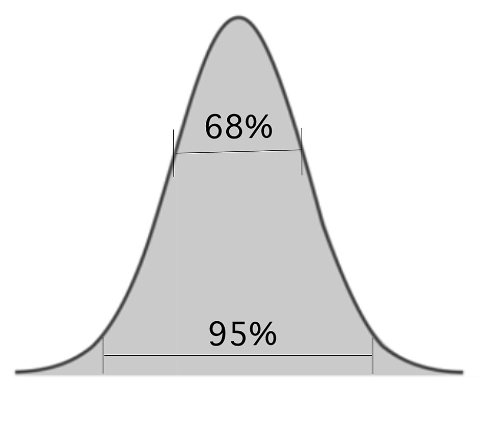 Bell curve with CI shaded (Image: Rohanukhade, CC0, via Wikimedia Commons)
Based on the PU BE Computer (PU) syllabus for Simulation and Modeling (CMP338), unit 7.
Discussion
Loading…