Correlation and Regression – Measures of Association and Predictive Modeling

1. Introduction to Correlation and Regression

Correlation and regression are the two pillars of bivariate analysis.

• Correlation quantifies the strength and direction of a linear relationship between two variables.
• Regression models the functional relationship, allowing prediction of one variable from another.

Both concepts rely on the same underlying data: paired observations $(x_i,y_i)$.

2. Covariance and Correlation Coefficient

2.1 Covariance

$$\mathrm{Cov}(X,Y)=\frac{1}{n-1}\sum _{i=1}^n(x_i-\bar{x})(y_i-\bar{y})$$

• Positive covariance → variables tend to increase together.
• Negative covariance → one variable tends to increase while the other decreases.
• Magnitude depends on units; hence not directly comparable across variable pairs.

2.2 Correlation Coefficient (Pearson’s $r$)

$$r=\frac{\mathrm{Cov}(X,Y)}{s_X{s}_Y}$$

where $s_X$ and $s_Y$ are sample standard deviations.

• $r\in [-1,1]$.
• $r=1$ or $-1$ indicates perfect linear relationship.
• $r=0$ indicates no linear relationship (but may still be non‑linear).

2.3 Worked Example – Promotional Expenses vs Sales

Compute $r$:

1. $\bar{x}=(44+61+10+12+15)/5=26.4$
2. $\bar{y}=(162+180+242+202+225)/5=204.6$
3. $\sum (x_i-\bar{x})(y_i-\bar{y})=1452.0$
4. $\sum (x_i-\bar{x}{)}^2=1332.8$
5. $\sum (y_i-\bar{y}{)}^2=13020.8$
6. $s_X=\sqrt{1332.8/4}=18.25$
7. $s_Y=\sqrt{13020.8/4}=57.04$
8. $r=1452.0/(18.25\times 57.04)=0.84$

Interpretation: A strong positive linear relationship; as promotional spend increases, sales tend to increase.

3. Coefficient of Determination ($R^2$)

$$R^2=r^2$$

• Represents the proportion of variance in $Y$ explained by $X$.
• $R^2=0.7056$ (from $r=0.84$) → 70.56 % of sales variation is explained by promotional spend.

3.1 Visualising $R^2$

4. Simple Linear Regression

4.1 Model

$$\hat{y}={\beta }_0+{\beta }_{1}x$$

• ${\beta }_1=r\frac{s_Y}{s_X}$
• ${\beta }_0=\bar{y}-{\beta }_1\bar{x}$

4.2 Calculating the Regression Coefficients

Using the example data:

1. ${\beta }_1=0.84\times \frac{57.04}{18.25}=2.62$
2. ${\beta }_0=204.6-2.62\times 26.4=132.5$

Regression equation:

$$\hat{y}=132.5+2.62x$$

4.3 Prediction Example

Predict sales for a promotional spend of Rs 200 000 (i.e., $x=200$ k):

$$\hat{y}=132.5+2.62\times 200=132.5+524=656.5\text{ (Rs ’00,000)}$$

Interpretation: A Rs 200 k spend is expected to generate approximately Rs 65.65 M in sales.

4.4 Flow of Regression Calculation (Mermaid)

flowchart TD
    "Collect Data" --> "Compute Means"
    "Compute Means" --> "Compute Deviations"
    "Compute Deviations" --> "Compute Covariance"
    "Compute Deviations" --> "Compute Variances"
    "Compute Covariance" --> "Compute r"
    "Compute Variances" --> "Compute s_X, s_Y"
    "Compute r" --> "Compute β1"
    "Compute β1" --> "Compute β0"
    "Compute β0" --> "Regression Equation"

4.5 Regression Output Table

5. Interpretation of Regression Output

5.1 Practical Decision

If the company can increase spend by Rs 50 k, expected sales increase ≈ $2.62\times 50=131$ k (Rs ’00,000).

6. Multiple Regression (Brief Overview)

When more than one predictor is available, the model becomes

$$\hat{y}={\beta }_0+{\beta }_1{x}_1+{\beta }_2{x}_2+\cdots +{\beta }_k{x}_k$$

• Allows control for confounding variables.
• Coefficients are interpreted as the effect of each predictor holding others constant.

6.1 Example (Hypothetical)

Regression yields $\hat{y}=100+1.5\text{TV}+2.0\text{Radio}$.

7. Assumptions and Diagnostics

7.1 Residual Plot

8. Advantages & Disadvantages

9. In the Real World

1. eSewa Transaction Analysis – Correlation between daily transaction volume and total transaction value shows a strong positive relationship ($r=0.88$). This helps eSewa forecast revenue peaks during festivals.
2. Daraz Promotional Spend – Regression of promotional expenses on sales (as in the worked example) is used by Daraz’s marketing team to allocate budgets across product categories.
3. Ncell Subscriber Growth – Correlation between advertising spend and subscriber additions ($r=0.75$) informs Ncell’s media buying strategy.

Worked Real‑World Example:
For Daraz, a promotional spend of Rs 200 k is predicted to yield Rs 65.65 M in sales, guiding the marketing budget for the upcoming sale event.

10. Exam Tip

• Know the formulas: covariance, correlation, regression coefficients, $R^2$.
• Practice data sets: compute $r$, $R^2$, ${\beta }_0$, ${\beta }_1$ by hand.
• Interpretation: always translate numbers into business implications.
• Assumptions: be ready to discuss how you would check them.
• Multiple choice: look for key terms like “explained variance” (R²) or “direction of association” (covariance).

11. Summary

Correlation and regression provide a quantitative backbone for business decision‑making. Covariance gives direction, correlation standardises it, and regression builds a predictive model. Mastery of these tools equips students to analyse marketing data, forecast sales, and optimize resource allocation in real Nepali and global enterprises.

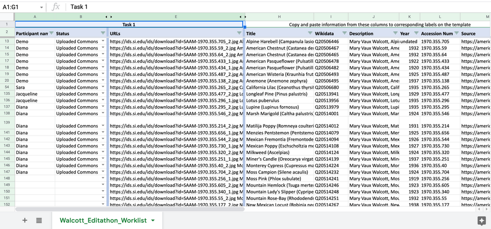A spreadsheet is the primary tool for organising paired data before analysis. (Image: Fuzheado, CC BY-SA 4.0, via Wikimedia Commons) A calculator is essential for quick computation of means, variances, and regression coefficients. (Image: LoMit, CC BY-SA 4.0, via Wikimedia Commons) Graph paper helps in visualising scatter plots and residuals before digital plotting. (Image: Mikus, CC BY-SA 4.0, via Wikimedia Commons)