Discrete and Continuous Probability Distributions – Key Concepts and Applications

Introduction

Probability distributions are the backbone of statistical inference. They formalise the randomness inherent in business data – from customer arrivals to transaction success rates. A random variable $X$ is a numerical description of an outcome of a random process.

• Discrete random variable: takes a countable set of values (e.g., number of sales in a day).
• Continuous random variable: takes any value in an interval (e.g., time between customer arrivals).

The distribution of $X$ is fully described by its probability mass function (pmf) for discrete variables or probability density function (pdf) for continuous variables.

Probability Mass Function (pmf)

For a discrete random variable $X$, the pmf $p(x)$ satisfies

$$p(x)=P(X=x),\sum _{x}p(x)=1,p(x)\ge 0.$$

The cumulative distribution function (cdf) is

$$F(x)=P(X\le x)=\sum _{t\le x}p(t).$$

Example: Bag of 20 Balls

A bag contains balls numbered 1 to 20. We want the probability that a randomly selected ball is a multiple of 3 or 7.

The shaded cells (X) represent favourable outcomes.
There are 8 favourable numbers (3, 6, 7, 9, 12, 14, 15, 18).

$$P(\text{multiple of 3 or 7})=\frac{8}{20}=\mathrm{0.4.}$$

Probability Density Function (pdf)

For a continuous random variable $X$, the pdf $f(x)$ satisfies

$$f(x)\ge 0,{\int }_{-\infty }^{\infty }f(x)dx=1.$$

The probability that $X$ falls in an interval $[a,b]$ is

$$P(a\le X\le b)={\int }_a^{b}f(x)dx.$$

The cdf is

$$F(x)={\int }_{-\infty }^{x}f(t)dt.$$

Key Discrete Distributions

Worked Example: Drawing Two Red Balls

Bag: 3 red, 2 black, 5 white (total 10). Two balls drawn without replacement.

$$P(\text{both red})=\frac{\left(\genfrac{}{}{0ex}{}{3}{2}\right)}{\left(\genfrac{}{}{0ex}{}{10}{2}\right)}=\frac{3}{45}=\mathrm{0.0667.}$$

Key Continuous Distributions

Worked Example: Normal Distribution

Daily income of part‑time staff: $\mu =1200$, $\sigma =120$. Find $P(1050\le X\le 1250)$.

Standardise:

$$Z=\frac{X-\mu }{\sigma }.$$

$$P(1050\le X\le 1250)=P\left(\frac{1050-1200}{120}\le Z\le \frac{1250-1200}{120}\right)=P(-1.25\le Z\le 0.42).$$

Using standard normal tables:

$$P(Z\le 0.42)\approx 0.6628,P(Z\le -1.25)\approx \mathrm{0.1056.}$$

$$P(1050\le X\le 1250)=0.6628-0.1056=\mathrm{0.5572.}$$

Expected Value and Variance

For a discrete random variable:

$$E[X]=\sum _{x}xp(x),\mathrm{Var}(X)=\sum _x(x-E[X]{)}^{2}p(x).$$

For a continuous random variable:

$$E[X]={\int }_{-\infty }^{\infty }xf(x)dx,\mathrm{Var}(X)={\int }_{-\infty }^{\infty }(x-E[X]{)}^{2}f(x)dx.$$

Worked Example: Given Distribution

$$\begin{array}{cccccc}x& 0& 1& 2& 3& 4\\ p(x)& 0.22& 0.18& 0.35& 0.15& 0.10\end{array}$$

Compute $E[X]$ and $\mathrm{Var}(X)$.

$$E[X]=0(0.22)+1(0.18)+2(0.35)+3(0.15)+4(0.10)=0+0.18+0.70+0.45+0.40=\mathrm{1.73.}$$

$$E[X^2]=0^2(0.22)+1^2(0.18)+2^2(0.35)+3^2(0.15)+4^2(0.10)=0+0.18+1.40+1.35+1.60=\mathrm{4.53.}$$

$$\mathrm{Var}(X)=E[X^2]-(E[X]{)}^2=4.53-(1.73{)}^2=4.53-2.99=\mathrm{1.54.}$$

Comparison: Discrete vs Continuous

Process of Selecting Balls – Flowchart

flowchart TD
  "Start"["Start"] --> "Draw first ball"
  "Draw first ball" --> "Check colour"
  "Check colour" -->|"Red"| "Draw second ball"
  "Check colour" -->|"Not red"| "End"
  "Draw second ball" --> "Check colour"
  "Check colour" -->|"Red"| "Success"
  "Check colour" -->|"Not red"| "End"

In the real world

1. eSewa (Digital Wallet) – Uses a Poisson distribution to model the number of transaction requests per second. The mean rate $\lambda$ is estimated from historical traffic; this informs server scaling decisions.
2. Daraz (E‑commerce) – The daily order value follows an approximate normal distribution. Marketing teams use the mean and standard deviation to set dynamic discount thresholds that maximise revenue.
3. Pathao (Ride‑hailing) – The inter‑arrival time of ride requests is modeled with an exponential distribution. The rate parameter $\lambda$ helps dispatch algorithms predict peak demand and allocate drivers efficiently.

Worked Real‑World Example

A bank wants to estimate the probability that a randomly chosen customer will take a loan of more than Rs. 500,000. Historical loan amounts are normally distributed with $\mu =350,000$ and $\sigma =120,000$.

$$P(X>500,000)=1-P\left(Z\le \frac{500,000-350,000}{120,000}\right)=1-P(Z\le 1.25)\approx 1-0.8944=\mathrm{0.1056.}$$

Thus, about 10.6 % of customers are expected to request loans above Rs. 500,000.

Exam tip

• Identify the type of distribution: discrete (pmf) vs continuous (pdf).
• Use the correct formula for probability, expectation, and variance.
• Check the parameters (e.g., $n,p$ for binomial; $\lambda$ for Poisson; $\mu ,\sigma$ for normal).
• Show all steps in calculations; write the formula you are using.
• Draw a small diagram (figure or mermaid) if the question involves a process or selection.
• Remember key properties: for normal distribution, use z‑scores; for Poisson, use the factorial term.

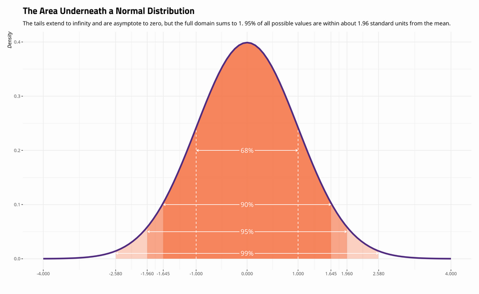Smooth bell‑shaped curve with mean and standard deviation labeled (Image: ssindhwani, CC BY-SA 4.0, via Wikimedia Commons)

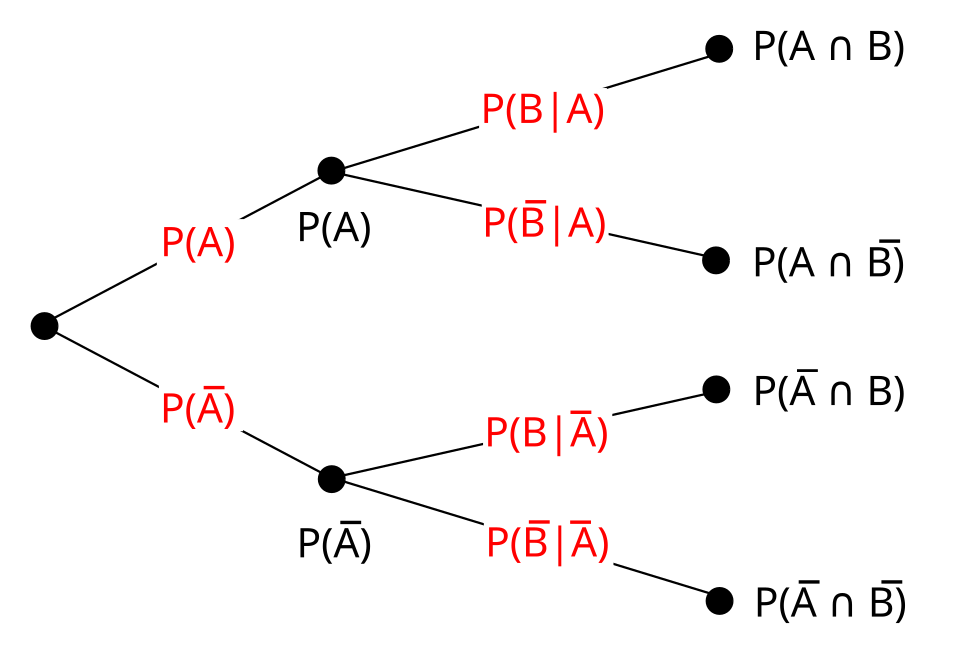Tree showing outcomes of drawing balls from a bag (Image: Gnathan87 (talk · contribs), CC0, via Wikimedia Commons)