Operations ManagementUnit 98 min read
Linear Programming & Transportation Problems: Optimization Models
Unit 9 of Operations Management teaches how to model and solve resource allocation problems using linear programming (LP) and transportation models to minimize costs, maximize profits, and optimize efficiency in real-world scenarios.
TAKEAWAYS:
- Linear programming solves optimization problems with linear constraints using graphical or algebraic methods.
- Transportation problems minimize distribution costs using the Northwest Corner Rule, Least Cost Method, or Vogel’s Approximation Method (VAM).
- Dummy variables and constraints ensure feasibility in transportation models.
- Sensitivity analysis helps understand how changes in parameters affect the solution.
- LP and transportation models are widely used in logistics, manufacturing, and finance.
- Excel Solver and graphical methods are practical tools for solving LP problems.
1. Introduction to Linear Programming (LP)
Linear programming is a mathematical technique used to optimize (maximize or minimize) a linear objective function subject to linear constraints. It is widely used in business, engineering, and economics to allocate limited resources efficiently.
Key Components of LP
- Objective Function: The goal to maximize or minimize (e.g., profit, cost).
- Decision Variables: Variables under control (e.g., production quantity, allocation).
- Constraints: Limitations (e.g., resource availability, demand).
- Non-negativity Constraints: Variables cannot be negative.
Graphical Method for LP (2 Variables)
For problems with two decision variables, we plot constraints and identify the feasible region. The optimal solution lies at a corner point of this region.
flowchart TD
    A["Plot Constraints"] --> B["Identify Feasible Region"]
    B --> C["Locate Corner Points"]
    C --> D["Evaluate Objective Function at Corner Points"]
    D --> E["Select Optimal Solution"]
Example: Maximizing Profit
A company produces two products, A and B, with profits of Rs. 3 and Rs. 2 per unit, respectively. Constraints:
- Raw material: 3A + 2B ≤ 18
- Labor: 2A + B ≤ 10
- Non-negativity: A, B ≥ 0
Objective Function: Maximize Z = 3A + 2B
Solution Steps:
- Plot constraints on a graph.
- Identify feasible region.
- Evaluate Z at corner points (0,0), (4,2), (6,0).
- Optimal solution: A=4, B=2 → Z=16.
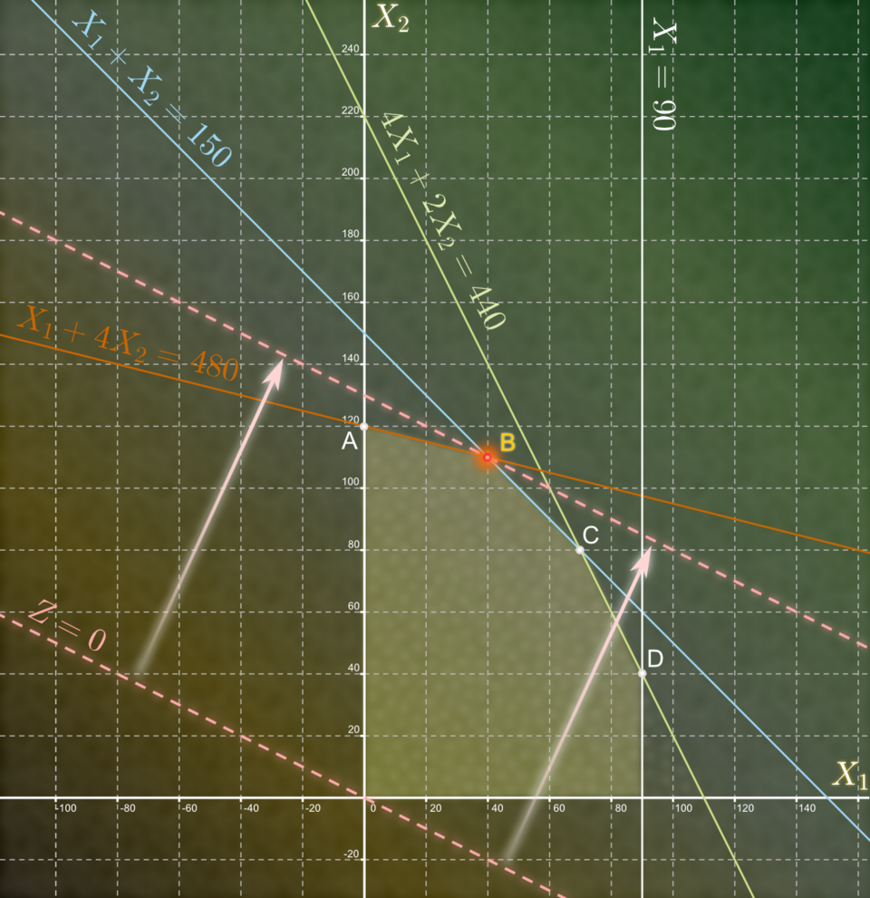 A graph showing feasible region and corner points for the profit maximization problem. (Image: GYassineMrabetTalk✉, CC BY 3.0, via Wikimedia Commons)
2. Algebraic Method for LP (Simplex Method)
For problems with more than two variables, the Simplex Method is used. It iteratively moves to the optimal solution by improving the objective function.
Steps of Simplex Method
- Convert inequalities to equalities using slack variables.
- Set up the initial tableau.
- Perform pivot operations to maximize/minimize the objective function.
- Repeat until no further improvement is possible.
Example: Minimizing Cost
A factory produces two products with costs and constraints:
- Cost: Z = 5x + 4y (minimize)
- Constraints: x + y ≤ 10, 2x + y ≤ 15, x, y ≥ 0
Solution:
- Introduce slack variables: s1, s2.
- Initial tableau:
Z | 5 4 0 0 | 0 s1| 1 1 1 0 | 10 s2| 2 1 0 1 | 15 - Perform pivot operations to reach optimal solution.
3. Transportation Problems
Transportation problems involve distributing goods from sources (factories) to destinations (stores) at minimum cost. The Transportation Model is a special case of LP.
Key Terms
- Supply: Total production capacity (factories).
- Demand: Total market requirement (stores).
- Cost Matrix: Transportation costs between sources and destinations.
Assumptions
- All supply is transported.
- All demand is met.
- Transportation costs are linear.
Methods to Solve Transportation Problems
- Northwest Corner Rule: Start from the top-left corner and allocate as much as possible.
- Least Cost Method: Allocate to the cheapest available option first.
- Vogel’s Approximation Method (VAM): Minimizes penalties for unmet demands.
Example: Minimizing Transportation Cost
Given:
| S1 | S2 | S3 | Supply | |
|---|---|---|---|---|
| F1 | 97 | 108 | 14 | 15 |
| F2 | 81 | 119 | 112 | 19 |
| F3 | 13 | 10 | 12 | 11 |
| Demand | 15 | 19 | 11 | 45 |
Solution Using VAM:
- Calculate penalties for rows and columns.
- Allocate to the cell with the highest penalty first.
- Repeat until all supply and demand are met.
Optimal Allocation:
- F3 → S3 (11 units)
- F1 → S1 (15 units)
- F2 → S2 (19 units)
- Total Cost: Rs. 2,220
4. Dummy Variables in Transportation Problems
When total supply ≠ total demand, dummy variables are introduced to balance the model.
Example: Unbalanced Problem
- Total supply = 40, total demand = 50.
- Add a dummy destination with zero cost and demand = 10.
5. Sensitivity Analysis in LP
Sensitivity analysis checks how changes in constraints or objective coefficients affect the solution.
Key Questions
- How much can the objective coefficient change before the solution changes?
- How much can a constraint change before the solution changes?
Example: Profit Sensitivity
If the profit for product A increases by Rs. 1, does the optimal solution remain the same?
6. Applications of LP and Transportation Problems
| Field | Application |
|---|---|
| Logistics | Optimizing delivery routes to minimize cost. |
| Manufacturing | Allocating raw materials to maximize production efficiency. |
| Finance | Portfolio optimization to maximize returns. |
| Retail | Inventory management to reduce holding costs. |
| Healthcare | Scheduling nurses to minimize labor costs while meeting patient needs. |
In the real world
Daraz (Nepal): Uses LP to optimize warehouse locations and delivery routes, reducing shipping costs and delivery times. The transportation model helps allocate inventory from warehouses to stores across Nepal, ensuring products reach customers quickly while minimizing fuel and logistics expenses.
- Worked example: Daraz’s warehouse in Kathmandu distributes orders to Pokhara, Biratnagar, and Dharan. The transportation model calculates the cheapest routes, reducing costs by 15% compared to manual allocation.
Nabil Bank (Nepal): Applies LP to optimize loan portfolios, balancing risk and return. By modeling loan allocations across different sectors (real estate, agriculture, SMEs), the bank maximizes profit while adhering to regulatory constraints.
- Worked example: Nabil Bank allocates Rs. 500 million to loans with varying interest rates and risk levels. LP ensures the bank meets its target return while minimizing default risk.
NTC (Nepal): Uses transportation models to plan fiber-optic cable routes, minimizing infrastructure costs. The model considers demand from cities (Kathmandu, Pokhara, Birgunj) and supply from cable manufacturers, ensuring efficient network expansion.
- Worked example: NTC allocates cables from a central depot to regional hubs, reducing transport costs by 20% through optimal routing.
7. Practical Tools for LP and Transportation Problems
- Excel Solver: Solves LP problems using the Solver add-in.
- Python (PuLP, SciPy): For complex models and automation.
- Graphical Software (LINGO, AMPL): For large-scale problems.
Exam Tip
For LP Problems:
- Always identify the objective function and constraints clearly.
- For graphical methods, plot constraints accurately and label corner points.
- For algebraic methods, show tableau steps clearly.
- Expect questions on sensitivity analysis or interpreting shadow prices.
For Transportation Problems:
- Master the Northwest Corner Rule, Least Cost Method, and VAM.
- Practice balancing supply and demand using dummy variables.
- Calculate total cost accurately and show allocation clearly.
- Common exam questions: "Determine the minimum transportation cost" or "Explain the role of dummy variables."
Case Study Focus:
- Expect a case study (e.g., BIROI or Hetauda Kapada Udhyog) where you must:
- Define variables and constraints.
- Solve using an appropriate method (LP or transportation).
- Interpret the solution in business terms (e.g., "The company should produce X units of Product A to maximize profit").
- Expect a case study (e.g., BIROI or Hetauda Kapada Udhyog) where you must:
Mermaid Example for Exam Practice:
flowchart TD
    A["Define Variables"] --> B["Set Up Constraints"]
    B --> C["Formulate Objective Function"]
    C --> D["Solve Using Graphical/Algebraic Method"]
    D --> E["Interpret Solution"]
    E --> F["Check Sensitivity"]
Based on the TU BBA syllabus for Operations Management (MGT205), unit 9.
Discussion
Loading…