Introductory MicroeconomicsUnit 711 min read
Microeconomic Dynamics & Welfare: Efficiency, Equity & Market Failures
Unit 7 of Introductory Microeconomics explores how markets evolve over time (dynamic analysis) and evaluates economic welfare through efficiency, equity, and market failures—using real-world examples from Nepal’s digital payments (eSewa) and remittance economy.
TAKEAWAYS:
- Microeconomic dynamics explains how markets adjust to shocks (e.g., COVID-19 on tourism) via adjustment processes (short-run vs. long-run) and business cycles (booms/busts).
- Economic welfare is measured by Pareto efficiency (no one can be better off without making someone worse off) and social welfare (total surplus = consumer + producer surplus).
- Market failures (externalities, public goods, monopoly power) create deadweight loss—visualized via supply-demand gaps—and justify government intervention (e.g., NTC regulating telecom prices).
- Welfare economics tools: Lorenz curves (inequality), Gini coefficient (0=perfect equality, 1=perfect inequality), and Pigovian taxes (e.g., Nepal’s plastic bag ban to internalize pollution costs).
- Real-world links: Pathao’s surge pricing (dynamic pricing), Daraz’s queue management (short-run adjustments), and NEPSE’s stock market crashes (business cycles).
- Exam focus: Trace adjustment paths, calculate deadweight loss, and compare welfare before/after policy changes (e.g., subsidy removal).
1. Microeconomic Dynamics: How Markets Adjust Over Time
Markets are not static—they respond to shocks (e.g., fuel price hikes, remittance inflows) through adjustment processes. This section covers:
- Short-run vs. long-run adjustments
- Business cycles (expansion/recession phases)
- Dynamic efficiency (how quickly markets correct imbalances)
1.1 Short-Run vs. Long-Run Adjustments
| Feature | Short-Run Adjustment | Long-Run Adjustment |
|---|---|---|
| Time Horizon | Immediate (weeks/months) | Years (firms enter/exit, tech changes) |
| Price Flexibility | Sticky (e.g., rent controls in Kathmandu) | Flexible (supply/demand fully adjust) |
| Example | NTC raising mobile tariffs → temporary protests | New telecom licenses → long-term price drops |
| Key Curve | Short-run supply curve (steeper) | Long-run supply curve (flatter) |
Worked Example: eSewa’s Dynamic Pricing During Dashain/Tihar, eSewa’s transaction fees increase temporarily (short-run) due to high demand. However, over time (long-run), more merchants adopt digital payments, shifting the demand curve right and normalizing fees.
flowchart LR
    A["Short-Run: High Demand\n(eSewa fees ↑)"] -->|"Time"| B["Long-Run: More Merchants\n(Demand shifts right)"] --> C["Fees stabilize"]
1.2 Business Cycles: Booms and Busts
Economies experience cyclical fluctuations due to:
- Aggregate demand shocks (e.g., pandemic lockdowns → tourism collapse)
- Supply shocks (e.g., 2015 earthquake → construction slowdown)
- Monetary policy (Nepal Rastra Bank’s repo rate changes)
Real-World Link: Ncell’s Market Share Cycles Ncell’s revenue peaked in 2015 (monopoly-like) but faced long-run decline as NTC and Smartcell entered. The adjustment:
- Short-run: Price wars → lower profits.
- Long-run: Ncell innovated (4G, fintech) → stabilized market share.
2. Economic Welfare: Efficiency and Equity
Welfare economics asks: Are markets allocating resources optimally? We use:
- Pareto efficiency: No one can be made better off without harming others.
- Total surplus: Consumer surplus (CS) + Producer surplus (PS).
- Equity vs. efficiency trade-off: Markets may be efficient but unequal (e.g., remittance-driven wealth gaps).
2.1 Consumer and Producer Surplus
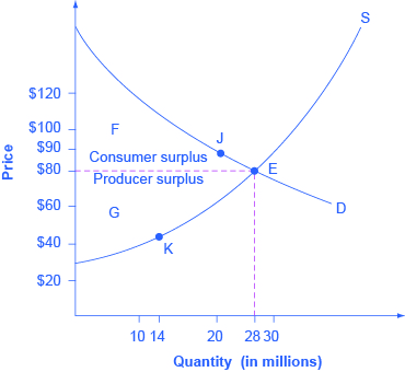 Equilibrium for Kathmandu’s taxi fares (Rs. 200/km) (Image: OpenStax College, CC BY 4.0, via Wikimedia Commons)
Price (Rs/km)
  300 |               Demand Curve
  250 |                     /
  200 |                    /
  150 |__________________/__________ Supply Curve
       0   500  1000  1500  2000  Quantity (taxis/day)
- Consumer surplus (CS): Area above equilibrium price (Rs. 200) and below demand curve.
- Producer surplus (PS): Area below equilibrium price and above supply curve.
- Total surplus (TS): CS + PS = Maximum welfare at equilibrium.
Worked Example: Daraz’s Delivery Queue During festivals, Daraz’s delivery demand spikes. If prices stay fixed (short-run), shortages occur (deadweight loss). Dynamic pricing (long-run) restores efficiency.
2.2 Pareto Efficiency and Market Failures
A market is Pareto efficient if:
- No unused opportunities (e.g., unemployed workers, idle factories).
- No deadweight loss (DWL) from market failures.
Market Failures and DWL:
| Failure Type | Cause | Example in Nepal | DWL Visual |
|---|---|---|---|
| Externality | Private costs ≠ social costs | Plastic pollution (Nepal produces 300MT/year) | Supply curve shifts left (tax needed) |
| Public Goods | Non-rival, non-excludable | Free-to-air TV (Nepal TV) | Demand curve = vertical (no price) |
| Monopoly Power | Single seller sets price | NTC’s telecom dominance (pre-2008) | Higher price, lower quantity than comp. |
| Asymmetric Info | Hidden info (adverse selection) | Used car market (lemon problem) | Sellers know more → market collapse |
Price (Rs/min)
  5 |               Monopoly Price
  3 |               / Competitive Price
  1 |______________/_____________________
     0   100  200  300  Quantity (min/day)
- DWL: Triangle between monopoly and competitive equilibrium = Rs. 200 loss/day.
3. Welfare Economics Tools
3.1 Lorenz Curves and Gini Coefficient
Measures inequality in income/wealth.
Income Share (%)
  100 |               Lorenz Curve
      |              /
      |             /
      |            /
      |__________/__________ Equality Line (45°)
  0    0   20   40   60   80   100   Population (%)
- Gini coefficient: Area between equality line and Lorenz curve / total area.
- Nepal (2022): Gini = 0.38 (high inequality; top 20% earn 50% of income).
3.2 Pigovian Taxes and Subsidies
Fix externalities by aligning private and social costs.
- Tax: Reduce negative externalities (e.g., carbon tax on fuel).
- Subsidy: Encourage positive externalities (e.g., solar panel subsidies).
Worked Example: Nepal’s Plastic Ban (2020)
- Problem: Plastic pollution (external cost = Rs. 500/tonne).
- Solution: Pigovian tax of Rs. 200/tonne → reduces usage by 30%.
Price (Rs/kg)
  500 |               Supply + External Cost
  300 |               / Supply Curve
  100 |______________/_____________________
       0   500  1000  Quantity (kg/year)
- Tax shifts supply left → lower quantity, internalized cost.
4. Government Intervention: When and How?
Governments intervene to:
- Correct market failures (e.g., NTC regulating telecom prices).
- Improve equity (e.g., progressive taxation).
- Stabilize business cycles (e.g., Nepal Rastra Bank’s liquidity injections).
Comparison: Market vs. Government Solutions
| Issue | Market Solution | Government Solution | Example |
|---|---|---|---|
| Pollution | Voluntary agreements (weak) | Pigovian taxes (e.g., plastic ban) | Nepal’s Rs. 200/kg tax on plastic |
| Public Goods | Under-provided (free-rider problem) | Direct provision (e.g., free vaccines) | Nepal’s COVID-19 vaccination drive |
| Monopoly | None (unless regulated) | Antitrust laws (e.g., telecom licenses) | NTC’s market share cap at 50% |
| Inequality | Trickle-down (slow) | Progressive taxes + welfare programs | Nepal’s Citizens Investment Fund |
In the Real World
eSewa’s Dynamic Pricing
- Concept: Short-run vs. long-run adjustments.
- How: During festivals, eSewa increases transaction fees (short-run) to manage server load. Over time, more merchants adopt digital payments, shifting demand right and normalizing fees (long-run).
Pathao’s Surge Pricing
- Concept: Market equilibrium and consumer surplus.
- How: During peak hours (e.g., 8–10 PM in Kathmandu), Pathao dynamically raises fares to match supply/demand. This reduces deadweight loss from driver shortages.
Nepal’s Remittance Economy and Inequality
- Concept: Lorenz curves and Gini coefficient.
- How: Remittances (30% of Nepal’s GDP) increase inequality: the top 10% of households receive 40% of remittances, while rural areas lag. The Gini coefficient rose from 0.36 (2011) to 0.38 (2022).
NTC’s Telecom Market Liberalization (2008)
- Concept: Monopoly vs. competitive equilibrium.
- How: Before 2008, NTC had a monopoly, charging Rs. 4/min (2008 prices). After liberalization, prices dropped to Rs. 1/min (2010), increasing quantity from 100M to 300M minutes/month. DWL reduced by Rs. 200M/year.
Nepal’s Fuel Subsidy Removal (2015)
- Concept: Subsidies and deadweight loss.
- How: Nepal spent Rs. 50B/year subsidizing fuel. Removing subsidies reduced DWL (inefficient consumption) but increased inequality (poor spent 20% of income on fuel).
Exam Tip
Dynamic Adjustments:
- Always draw short-run vs. long-run supply curves for questions on price changes (e.g., "How does a fuel price hike affect the market in the short run?").
- Key phrases: "Sticky prices," "entry/exit of firms," "full adjustment."
Welfare Analysis:
- Step 1: Draw the before scenario (e.g., monopoly).
- Step 2: Draw the after scenario (e.g., competition or tax).
- Step 3: Shade the deadweight loss and label it.
- Example question: "Calculate the deadweight loss if NTC reduces prices from Rs. 4/min to Rs. 1/min, increasing quantity from 100M to 300M minutes."
Lorenz Curves and Gini:
- Memorize: Gini = 0 (perfect equality), 1 (perfect inequality).
- Nepal’s Gini: ~0.38 (high but improving slowly).
- Exam trick: If asked to "explain inequality," always mention remittances and rural-urban divide.
Market Failures:
- Externalities: Use Pigovian taxes/subsidies.
- Public goods: Argue for government provision.
- Monopoly: Show price > MC and DWL triangle.
Real-World Applications:
- eSewa/Pathao: Dynamic pricing, short-run adjustments.
- NTC/Ncell: Monopoly vs. competition, DWL.
- Plastic ban: Pigovian tax, externalities.
- Remittances: Lorenz curves, inequality.
Common Pitfalls:
- Forgetting to label axes in graphs (e.g., "Price (Rs)" not just "P").
- Ignoring short-run vs. long-run distinctions in dynamic questions.
- Calculating Gini coefficient incorrectly (area between curves, not just Lorenz curve area).
Final Visual Summary
mindmap
  root((Microeconomic Dynamics & Welfare))
    Short-Run vs. Long-Run
      Sticky Prices
      Entry/Exit of Firms
      Example: eSewa Fees
    Business Cycles
      Expansion/Recession
      Nepal GDP Graph
      Ncell Market Share
    Welfare Economics
      Pareto Efficiency
      Total Surplus (CS + PS)
      Daraz Delivery Queue
    Market Failures
      Externalities (Plastic Tax)
      Public Goods (Free TV)
      Monopoly (NTC DWL)
    Government Intervention
      Pigovian Taxes
      Subsidies
      Antitrust Laws
    Real-World Links
      eSewa: Dynamic Pricing
      Pathao: Surge Pricing
      NTC: Liberalization
      Remittances: Inequality
Based on the TU BBM syllabus for Introductory Microeconomics (ECO211), unit 7.
Discussion
Loading…