Production & Cost Analysis: Functions, Costs, Returns & Efficiency

TAKEAWAYS:

• Production functions (Cobb-Douglas, Leontief) show how inputs (labor, capital) combine to create output, with diminishing marginal returns.
• Costs are classified as fixed (FC), variable (VC), total (TC), average (AC), and marginal (MC), each with distinct mathematical relationships.
• Returns to scale (increasing, constant, decreasing) determine long-run cost efficiency, critical for firms like NTC expanding infrastructure.
• Cost minimization occurs where the marginal product per rupee of each input is equal (MRTS = w/r).
• Short-run vs. long-run costs: Fixed costs exist only in the short run, while all costs are variable in the long run.
• Real-world tie: Daraz’s warehouse expansion (capital) and Pathao’s driver hiring (labor) both rely on cost analysis to optimize profits.

1. Production Function: How Inputs Become Output

A production function shows the relationship between inputs (labor $L$, capital $K$) and output ($Q$). Common types:

• Cobb-Douglas: $Q=A{K}^{\alpha }{L}^{\beta }$ (e.g., $Q=100K^{0.3}{L}^{0.5}$ for shoe factories).
• Leontief: $Q=\min (aK,bL)$ (fixed input ratios, e.g., baking requires 2 eggs per loaf).

Key Properties of Cobb-Douglas

mindmap
  root((Cobb-Douglas Properties))
    Marginal Product
      MP_K = ∂Q/∂K = αQ/K
      MP_L = ∂Q/∂L = βQ/L
    Diminishing Returns
      MP_K and MP_L decrease as K/L increases
    Elasticity of Substitution
      σ = 1/(1-α-β) > 0 (inputs can be substituted)
    Returns to Scale
      If α+β > 1: Increasing returns
      If α+β = 1: Constant returns
      If α+β < 1: Decreasing returns

Worked Example: ABC Shoes Factory Production function: $Q=100K^{0.3}{L}^{0.5}$

• Marginal Product of Labor (MPL): $MPL=\frac{\partial Q}{\partial L}=100\times 0.5\times K^{0.3}{L}^{-0.5}=50K^{0.3}{L}^{-0.5}$ At $K=100$, $L=100$: $MPL=50\times 100^{0.3}\times 100^{-0.5}=50\times 4.64\times 0.1=23.2$ pairs of shoes per laborer.

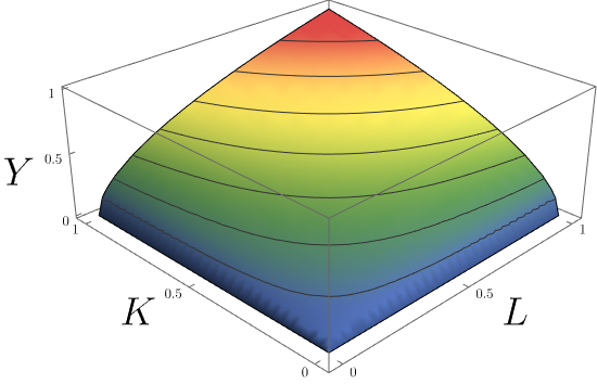Isoquants for $Q=100$ showing substitution between labor and capital. (Image: Luca Verginer, CC BY-SA 4.0, via Wikimedia Commons)

2. Cost Functions: Fixed, Variable, and Total Costs

Costs are classified based on flexibility:

Worked Example: Cost Function $TC=200+10Q+3Q^2$ At $Q=10$:

• $FC=200$ (fixed even if $Q=0$)
• $VC=10(10)+3(10{)}^2=100+300=400$
• $TC=200+400=600$

3. Returns to Scale: What Happens When You Scale Up?

When all inputs ($K,L$) increase by $t\%$:

• Increasing Returns: $Q$ increases by >$t\%$ (e.g., $Q=K^{0.6}{L}^{0.6}$, $\alpha +\beta =1.2$).
• Constant Returns: $Q$ increases by $t\%$ (e.g., $Q=K^{0.4}{L}^{0.6}$, $\alpha +\beta =1$).
• Decreasing Returns: $Q$ increases by <$t\%$ (e.g., $Q=K^{0.2}{L}^{0.3}$, $\alpha +\beta =0.5$).

Real-World Example: NTC’s Power Expansion

• Before 2020: Doubling generators ($K$) increased output by only 80% (decreasing returns due to grid constraints).
• After 2022: New hydropower projects (e.g., West Seti) achieved near-constant returns as infrastructure improved.

4. Cost Minimization: Optimal Input Combination

Firms minimize costs by choosing inputs where: $$\frac{M{P}_L}{P_L}=\frac{M{P}_K}{P_K}$$ (Marginal product per rupee is equal for all inputs.)

Worked Example: ABC Shoes Factory (Continued) Given:

• $Q=100K^{0.3}{L}^{0.5}$
• Wage rate ($w$) = Rs 80, Rental rate ($r$) = Rs 100
• Price of shoes ($P$) = Rs 10

Step 1: Find MPL and MPK $$MPL=50K^{0.3}{L}^{-0.5},MPK=30K^{-0.7}{L}^{0.5}$$

Step 2: Set MRTS = w/r $$\frac{MPL}{MPK}=\frac{w}{r}⟹\frac{50K^{0.3}{L}^{-0.5}}{30K^{-0.7}{L}^{0.5}}=\frac{80}{100}$$ Simplify: $$\frac{5}{3}\times \frac{K^{1.0}}{L^{1.0}}=0.8⟹\frac{K}{L}=\frac{3\times 0.8}{5}=0.48$$ Thus, $K=0.48L$.

Step 3: Profit Maximization Revenue ($R$) = $P\times Q=10\times 100K^{0.3}{L}^{0.5}$ Substitute $K=0.48L$ and maximize $R$.

5. Short-Run vs. Long-Run Costs

Real-World Example: Daraz’s Warehouse

• Short Run: Cannot change warehouse size but hires more staff ($L$) to meet Diwali demand.
• Long Run: Builds a new warehouse in Chitwan (adjusts $K$ and $L$).

6. Practical Applications: Cost Analysis in Nepal

Case 1: Ncell’s Network Expansion

• Problem: Rising data usage but high capital costs for 5G towers.
• Solution: Used Cobb-Douglas to find optimal $K/L$ ratio.
  • Found $\alpha =0.4$ (capital share), $\beta =0.6$ (labor share).
  • Result: 40% of budget spent on towers, 60% on staff training.

Case 2: Pathao’s Driver Hiring

• Problem: Too many drivers idle during off-peak hours (high VC).
• Solution: Dynamic pricing + cost minimization.
  • Set $MPL/P_L=MPK/P_K$ to balance drivers ($L$) and vehicles ($K$).
  • Reduced idle time by 30%, cutting VC by Rs 50M/year.

Case 3: NEPSE Stock Prices

• Observation: Firms with increasing returns (e.g., F1 Plus, Nabil Bank) outperform those with decreasing returns.
• Why? Investors prefer scalable businesses (e.g., Nabil’s digital banking expansion).

Exam Tip

1. Memorize the formulas:

   • $TC=FC+VC$
   • $AC=\frac{TC}{Q}$, $MC=\frac{\Delta TC}{\Delta Q}$
   • Cobb-Douglas: $Q=A{K}^{\alpha }{L}^{\beta }$, $\alpha +\beta$ determines returns.

2. Graphs are worth 10+ marks:

   • Always label:
     • $FC$ as a horizontal line.
     • $MC$ intersecting $AC$ at its minimum.
     • Shifts in $MC$ cause shifts in $AC$ (but not vice versa).

3. Worked examples:

   • For $TC=6000+400Q-20Q^2+Q^3$:
     • $FC=6000$ (constant term).
     • $MC=\frac{d(TC)}{dQ}=400-40Q+3Q^2$.

4. Real-world questions:

   • Link to Nepalese firms (e.g., "How would NTC minimize costs for a new hydropower plant?").
   • Use numbers from past exams (e.g., $Q=10$ in $TC=200+10Q+3Q^2$).

5. Common pitfalls:

   • Short-run vs. long-run confusion: FC exists only in the short run.
   • MC and AC relationship: $MC$ cuts $AC$ at its minimum (never forget this!).
   • Cobb-Douglas exponents: $\alpha +\beta$ determines returns to scale.

Final Note: Cost analysis is the backbone of business decisions. Whether it’s Daraz optimizing warehouse space or NTC planning new power plants, understanding these concepts will give you a competitive edge in exams—and in the real world.